
How Much Computational Power Does It Take to Match the Human Brain?
By Joseph Carlsmith
Editor’s note: This article was published under our former name, Open Philanthropy. Some content may be outdated. You can see our latest writing here.
Open Philanthropy is interested in when AI systems will be able to perform various tasks that humans can perform (“AI timelines”). To inform our thinking, I investigated what evidence the human brain provides about the computational power sufficient to match its capabilities. This is the full report on what I learned. A medium-depth summary is available here. The executive summary below gives a shorter overview.
Introduction
Executive summary
Let’s grant that in principle, sufficiently powerful computers can perform any cognitive task that the human brain can. How powerful is sufficiently powerful? I investigated what we can learn from the brain about this. I consulted with more than 30 experts, and considered four methods of generating estimates, focusing on floating point operations per second (FLOP/s) as a metric of computational power.
These methods were:
- Estimate the FLOP/s required to model the brain’s mechanisms at a level of detail adequate to replicate task-performance (the“mechanistic method”).[1]The names “mechanistic method” and “functional method” were suggested by our technical advisor Dr. Dario Amodei, though he uses a somewhat more specific conception of the mechanistic method. Sandberg and Bostrom (2008) also distinguish between “straightforward multiplicate estimates” … Continue reading
- Identify a portion of the brain whose function we can already approximate with artificial systems, and then scale up to a FLOP/s estimate for the whole brain (the “functional method”).
- Use the brain’s energy budget, together with physical limits set by Landauer’s principle, to upper-bound required FLOP/s (the “limit method”).
- Use the communication bandwidth in the brain as evidence about its computational capacity (the “communication method”). I discuss this method only briefly.
None of these methods are direct guides to the minimum possible FLOP/s budget, as the most efficient ways of performing tasks need not resemble the brain’s ways, or those of current artificial systems. But if sound, these methods would provide evidence that certain budgets are, at least, big enough (if you had the right software, which may be very hard to create – see discussion in section 1.3).[2]Here I am using “software” in a way that includes trained models in addition to hand-coded programs. Some forms of hardware (including neuromorphic hardware – see Mead (1989)) complicate traditional distinctions between hardware and software, but the broader consideration at stake here – … Continue reading
Here are some of the numbers these methods produce, plotted alongside the FLOP/s capacity of some current computers.

These numbers should be held lightly. They are back-of-the-envelope calculations, offered alongside initial discussion of complications and objections. The science here is very far from settled.
For those open to speculation, though, here’s a summary of what I’m taking away from the investigation:
- Mechanistic method estimates suggesting that 1013-1017 FLOP/s is enough to match the human brain’s task-performance seem plausible to me. This is partly because various experts are sympathetic to these estimates (others are more skeptical), and partly because of the direct arguments in their support. Some considerations from this method point to higher numbers; and some, to lower numbers. Of these, the latter seem to me stronger.[3] Though it also seems easier, in general, to show that X is enough, than that X is strictly required – an asymmetry present throughout the report.
- I give less weight to functional method estimates, primarily due to uncertainties about (a) the FLOP/s required to fully replicate the functions in question, (b) what the relevant portion of the brain is doing (in the case of the visual cortex), and (c) differences between that portion and the rest of the brain (in the case of the retina). However, I take estimates based on the visual cortex as some weak evidence that the mechanistic method range above (1013-1017 FLOP/s) isn’t much too low. Some estimates based on recent deep neural network models of retinal neurons point to higher numbers, but I take these as even weaker evidence.
- I think it unlikely that the required number of FLOP/s exceeds the bounds suggested by the limit method. However, I don’t think the method itself airtight. Rather, I find some arguments in the vicinity persuasive (though not all of them rely directly on Landauer’s principle); various experts I spoke to (though not all) were quite confident in these arguments; and other methods seem to point to lower numbers.
- Communication method estimates may well prove informative, but I haven’t vetted them. I discuss this method mostly in the hopes of prompting further work.
Overall, I think it more likely than not that 1015 FLOP/s is enough to perform tasks as well as the human brain (given the right software, which may be very hard to create). And I think it unlikely (<10%) that more than 1021 FLOP/s is required.[4]The probabilities reported here should be interpreted as subjective levels of confidence or “credences,” not as claims about objective frequencies, statistics, or “propensities” (see Peterson (2009), Chapter 7, for discussion of various alternative interpretations of probability … Continue reading But I’m not a neuroscientist, and there’s no consensus in neuroscience (or elsewhere).
I offer a few more specific probabilities, keyed to one specific type of brain model, in the appendix.[5]I focus on this model in particular because I think it fits best with the mechanistic method evidence I’ve thought about most and take most seriously. Offering specific probabilities keyed to the minimum FLOP/s sufficient for task-performance, by contrast, requires answering further questions … Continue reading My current best-guess median for the FLOP/s required to run that particular type of model is around 1015 (note that this is not an estimate of the FLOP/s uniquely “equivalent” to the brain – see discussion in section 1.6).
As can be seen from the figure above, the FLOP/s capacities of current computers (e.g., a V100 at ~1014 FLOP/s for ~$10,000, the Fugaku supercomputer at ~4×10¹⁷ FLOP/s for ~$1 billion) cover the estimates I find most plausible.[6]See here for V100 prices (currently ~$8,799); and here the $1 billion Fugaku pricetag: “The six-year budget for the system and related technology development totaled about $1 billion, compared with the $600 million price tags for the biggest planned U.S. systems.” Fugaku FLOP/s performance … Continue reading However:
- Computers capable of matching the human brain’s task performance would also need to meet further constraints (for example, constraints related to memory and memory bandwidth).
- Matching the human brain’s task-performance requires actually creating sufficiently capable and computationally efficient AI systems, and I do not discuss how hard this might be (though note that training an AI system to do X, in machine learning, is much more resource-intensive than using it to do X once trained).[7] See discussion in Section 1.3 below.
So even if my best-guesses are right, this does not imply that we’ll see AI systems as capable as the human brain anytime soon.
Acknowledgements: This report emerged out of Open Philanthropy’s engagement with some arguments suggested by one of our technical advisors, Dario Amodei, in the vein of the mechanistic/functional methods (see citations throughout the report for details). However, my discussion should not be treated as representative of Dr. Amodei’s views; the project eventually broadened considerably; and my conclusions are my own. My thanks to Dr. Amodei for prompting the investigation, and to Open Philanthropy’s technical advisors Paul Christiano and Adam Marblestone for help and discussion with respect to different aspects of the report. I am also grateful to the following external experts for talking with me. In neuroscience: Stephen Baccus, Rosa Cao, E.J. Chichilnisky, Erik De Schutter, Shaul Druckmann, Chris Eliasmith, davidad (David A. Dalrymple), Nick Hardy, Eric Jonas, Ilenna Jones, Ingmar Kanitscheider, Konrad Kording, Stephen Larson, Grace Lindsay, Eve Marder, Markus Meister, Won Mok Shim, Lars Muckli, Athanasia Papoutsi, Barak Pearlmutter, Blake Richards, Anders Sandberg, Dong Song, Kate Storrs, and Anthony Zador. In other fields: Eric Drexler, Owain Evans, Michael Frank, Robin Hanson, Jared Kaplan, Jess Riedel, David Wallace, and David Wolpert. My thanks to Dan Cantu, Nick Hardy, Stephen Larson, Grace Lindsay, Adam Marblestone, Jess Riedel, and David Wallace for commenting on early drafts (or parts of early drafts) of the report; to six other neuroscientists (unnamed) for reading/commenting on a later draft; to Ben Garfinkel, Catherine Olsson, Chris Sommerville, and Heather Youngs for discussion; to Nick Beckstead, Ajeya Cotra, Allan Dafoe, Tom Davidson, Owain Evans, Katja Grace, Holden Karnofsky, Michael Levine, Luke Muehlhauser, Zachary Robinson, David Roodman, Carl Shulman, Bastian Stern, and Jacob Trefethen for valuable comments and suggestions; to Charlie Giattino, for conducting some research on the scale of the human brain; to Asya Bergal for sharing with me some of her research on Landauer’s principle; to Jess Riedel for detailed help with the limit method section; to AI Impacts for sharing some unpublished research on brain-computer equivalence; to Rinad Alanakrih for help with image permissions; to Robert Geirhos, IEEE, and Sage Publications for granting image permissions; to Jacob Hilton and Gregory Toepperwein for help estimating the FLOP/s costs of different models; to Hannah Aldern and Anya Grenier for help with recruitment; to Eli Nathan for extensive help with the website and citations; to Nik Mitchell, Andrew Player, Taylor Smith, and Josh You for help with conversation notes; and to Nick Beckstead for guidance and support throughout the investigation.
Caveats
(This section discusses some caveats about the report’s epistemic status, and some notes on presentation. Those eager for the main content, however uncertain, can skip to section 1.3.)
Some caveats:
- Little if any of the evidence surveyed in this report is particularly conclusive. My aim is not to settle the question, but to inform analysis and decision-making that must proceed in the absence of conclusive evidence, and to lay groundwork for future work.
- I am not an expert in neuroscience, computer science, or physics (my academic background is in philosophy).
- I sought out a variety of expert perspectives, but I did not make a rigorous attempt to ensure that the experts I spoke to were a representative sample of opinion in the field. Various selection effects influencing who I interviewed plausibly correlate with sympathy towards lower FLOP/s requirements.[8]Selection effects include: expertise related to an issue relevant to the report, willingness to talk with me about the subject, recommendation by one of the other experts I spoke with as a possible source of helpful input, and connection (sometimes a few steps removed) with the professional and … Continue reading
- For various reasons, the research approach used here differs from what might be expected in other contexts. Key differences include:
- I give weight to intuitions and speculations offered by experts, as well as to factual claims by experts that I have not independently verified (these are generally documented in conversation notes approved by the experts themselves).
- I report provisional impressions from initial research.
- My literature reviews on relevant sub-topics are not comprehensive.
- I discuss unpublished papers where they appear credible.
- My conclusions emerge from my own subjective synthesis of the evidence I engaged with.
- There are ongoing questions about the baseline reliability of various kinds of published research in neuroscience and cognitive science.[9]See Poldrack et al. (2017); Vul and Pashler (2017); Uttal (2012); Button et al. (2013); Szucs and P.A. loannidis (2017); and Carp (2012). And see also Muehlhauser (2017b), Appendix Z.8, for discussion of his reasons for default skepticism of published studies. My thanks to Luke Muehlhauser … Continue reading I don’t engage with this issue explicitly, but it is an additional source of uncertainty.
A few other notes on presentation:
- I have tried to keep the report accessible to readers with a variety of backgrounds.
- The endnotes are frequent and sometimes lengthy, and they contain more quotes and descriptions of my research process than is academically standard. This is out of an effort to make the report’s reasoning transparent to readers. However, the endnotes are not essential to the main content, and I suggest only reading them if you’re interested in more details about a particular point.
- I draw heavily on non-verbatim notes from my conversations with experts, made public with their approval and cited/linked in endnotes. These notes are also available here.
- I occasionally use the word “compute” as a shorthand for “computational power.”
- Throughout the rest of the report, I use a form of scientific notation, in which “XeY” means “X×10Y.” Thus, 1e6 means 1,000,000 (a million); 4e8 means 400,000,000 (four hundred million); and so on. I also round aggressively.
Context
(This section briefly describes what prompts Open Philanthropy’s interest in the topic of this report. Those primarily interested in the main content can skip to Section 1.4.)
This report is part of a broader effort at Open Philanthropy to investigate when advanced AI systems might be developed (“AI timelines”) – a question that we think decision-relevant for our grant-making related to potential risks from advanced AI.[10] This effort is itself part of a project at Open Philanthropy currently called Worldview Investigations, which aims to investigate key questions informing our grant-making. But why would an interest in AI timelines prompt an interest in the topic of this report in particular?
Some classic analyses of AI timelines (notably, by Hans Moravec and Ray Kurzweil) emphasize forecasts about when available computer hardware will be “equivalent,” in some sense (see section 1.6 for discussion), to the human brain.[11] See, for example, Moravec (1998), chapter 2; and Kurzweil (2005), chapter 3. See this list from AI Impacts for related forecasts.

A basic objection to predicting AI timelines on this basis alone is that you need more than hardware to do what the brain does.[12]See, for example, Malcolm (2000); Lanier (2000) (“Belief # 5”); Russell (2019) (p. 78). AI Impacts offers a framework that I find helpful, which uses indifference curves indicating which combinations hardware and software capability yield the same overall task-performance. This framework … Continue reading In particular, you need software to run on your hardware, and creating the right software might be very hard (Moravec and Kurzweil both recognize this, and appeal to further arguments).[13] Moravec argues here that “under current circumstances, I think computer power is the pacing factor for AI” (see his second reply to Robin Hanson). Kurzweil (2005) devotes all of Chapter 4 to the question of software.
In the context of machine learning, we can offer a more specific version of this objection: the hardware required to run an AI system isn’t enough; you also need the hardware required to train it (along with other resources, like data).[14] For example: a ResNet-152 uses ~1e10 FLOP to classify an image, but took ~1e19 FLOP (a billion times more) to train, according to Hernandez and Amodei (2018) (see appendix, though see also Hernandez and Brown (2020) for discussion of decreasing training costs for vision models over time). And training a system requires running it a lot. DeepMind’s AlphaGo Zero, for example, trained on ~5 million games of Go.[15]Silver et al. (2017): “Over the course of training, 4.9 million games of self-play were generated” (see “Empirical analysis of AlphaGo Zero training”). A bigger version of the model trained on 29 million games. See Kaplan et al. (2020) and Hestness et al. (2017) for more on the scaling … Continue reading
Note, though, that depending on what sorts of task-performance will result from what sorts of training, a framework for thinking about AI timelines that incorporated training requirements would start, at least, to incorporate and quantify the difficulty of creating the right software more broadly.[16] The question of what sorts of task-performance will result from what sorts of training is centrally important in this context, and I am not here assuming any particular answers to it. This is because training turns computation, data, and other resources into software you wouldn’t otherwise know how to make.
What’s more, the hardware required to train a system is related to the hardware required to run it.[17] The fact that training a model requires running it a lot makes this clear. But there are also more complex relationships between e.g. model size and amount of training data. See Kaplan et al. (2020) and Hestness et al. (2017). This relationship is central to Open Philanthropy’s interest in the topic of this report, and to an investigation my colleague Ajeya Cotra has been conducting, which draws on my analysis. That investigation focuses on what brain-related FLOP/s estimates, along with other estimates and assumptions, might tell us about when it will be feasible to train different types of AI systems. I don’t discuss this question here, but it’s an important part of the context. And in that context, brain-related hardware estimates play a different role than they do in forecasts like Moravec’s and Kurzweil’s.
FLOP/s basics
(This section discusses what FLOP/s are, and why I chose to focus on them. Readers familiar with FLOP/s and happy with this choice can skip to Section 1.5.)
Computational power is multidimensional – encompassing, for example, the number and type of operations performed per second, the amount of memory stored at different levels of accessibility, and the speed with which information can be accessed and sent to different locations.[18]See e.g. Dongerra et al. (2003): “the performance of a computer is a complicated issue, a function of many interrelated quantities. These quantities include the application, the algorithm, the size of the problem, the high-level language, the implementation, the human level of effort used to … Continue reading
This report focuses on operations per second, and in particular, on “floating point operations.”[19]An operation, here, is an abstract mapping from inputs to outputs that can be implemented by a computer, and that is treated as basic for the purpose of the analysis in question (see Schneider and Gersting (2018) (p. 96-100)). A FLOP is itself composed out of a series of much simpler logic … Continue reading These are arithmetic operations (addition, subtraction, multiplication, division) performed on a pair of floating point numbers – that is, numbers represented as a set of significant digits multiplied by some other number raised to some exponent (like scientific notation). I’ll use “FLOPs” to indicate floating point operations (plural), and “FLOP/s” to indicate floating point operations per second.
My central reason for focusing on FLOP/s is that various brain-related FLOP/s estimates are key inputs to the framework for thinking about training requirements, mentioned above, that my colleague Ajeya Cotra has been investigating, and they were the focus of Open Philanthropy’s initial exploration of this topic, out of which this report emerged. Focusing on FLOP/s in particular also limits the scope of what is already a fairly broad investigation; and the availability of FLOP/s is one key contributor to recent progress in AI.[20]See e.g. Kahn and Mann (2020): “The success of modern AI techniques relies on computation on a scale unimaginable even a few years ago. Training a leading AI algorithm can require a month of computing time and cost $100 million” (p. 3); and Geoffrey Hinton’s comments in Lee (2016): “In … Continue reading
Still, the focus on FLOP/s is a key limitation of this analysis, as other computational resources are just as crucial to task-performance: if you can’t store the information you need, or get it where it needs to be fast enough, then the units in your system that perform FLOPs will be some combination of useless and inefficiently idle.[21]I say a little bit about communication bandwidth in Section 5. See Sandberg and Bostrom (2008) (p. 84-85), for a literature review of memory estimates. See Open Philanthropy’s non-verbatim notes from a conversation with Dr. Adam Marblestone] (“FLOP/s”) for some discussion of other … Continue reading Indeed, my understanding is that FLOP/s are often not the relevant bottleneck in various contexts related to AI and brain modeling.[22]Eugene Izhikevich, for example, reports that in running his brain simulation, he did not have the memory required to store all of the synaptic weights (10,000 terabytes), and so had to regenerate the anatomy of his simulated brain every time step; and Stephen Larson suggested that one of the … Continue reading And further dimensions an AI system’s implementation, like hardware architecture, can introduce significant overheads, both in FLOP/s and other resources.[23]From Open Philanthropy’s non-verbatim notes from a conversation with Dr. Adam Marblestone: “the architecture of a given computer (especially e.g. a standard von Neumann architecture) might create significant overhead. For example, the actual brain co-locates long-term memory and computing. If … Continue reading
Ultimately, though, once other computational resources are in place, and other overheads have mostly been eliminated or accounted for, you need to actually perform the FLOP/s that a given time-limited computation requires. In order to isolate this quantity, I proceed on the idealizing assumption that non-FLOP resources are available in amounts adequate to make full use of all of the FLOP/s in question (but not in unrealistically extreme abundance), without significant overheads.[24]An example of “unrealistically extreme abundance” would be the type of abundance of memory required by a giant look-up table. Even bracketing such obviously extreme scenarios, though, it seems possible that trade-offs between FLOP/s and other computational resources might complicate talk about … Continue reading All talk of the “FLOP/s sufficient to X” assumes this caveat.
This means you can’t draw conclusions about which concrete computers can replicate human-level task performance directly from the FLOP/s estimates in this report, even if you think those estimates credible. Such computers will need to meet further constraints.[25] See Ananthanarayanan et al. (2009) for discussion of the hardware complexities involved in brain simulation.
Note, as well, that these estimates do not depend on the assumption that the brain performs operations analogous to FLOPs, or on any other similarities between brain architectures and computer architectures.[26]Objections focused on general differences between brains and various human-engineered computers (e.g., the brain lacks a standardized clock, the brain is very parallel, the brain is analog, the brain is stochastic, the brain is chaotic, the brain is embodied, the brain’s memory works differently, … Continue reading The report assumes that the tasks the brain performs can also be performed using a sufficient number of FLOP/s, but the causal structure in the brain that gives rise to task-performance could in principle take a wide variety of unfamiliar forms.
Neuroscience basics
(This section reviews some of the neural mechanisms I’ll be discussing, in an effort to make the report’s content accessible to readers without a background in neuroscience.[27] My impression is that the content reviewed here is basically settled science, though see Section 1.5.1 for discussion of various types of ongoing neuroscientific uncertainty. Those familiar with signaling mechanisms in the brain – neurons, neuromodulators, gap junctions – can skip to Section 1.5.1).
The human brain contains around 100 billion neurons, and roughly the same number of non-neuronal cells.[28]Azevedo et al. (2009): “We find that the adult male human brain contains on average 86.1 ± 8.1 billion NeuN-positive cells (“neurons”) and 84.6 ± 9.8 billion NeuN-negative (“nonneuronal”) cells” (532). My understanding is that the best available method of counting neurons is … Continue reading Neurons are cells specialized for sending and receiving various types of electrical and chemical signals, and other non-neuronal cells send and receive signals as well.[29]I do not have a rigorous definition of “signaling” between cells, though there may be one available. A central example would be when one cell has a specialized mechanism for sending out a particular type of chemical to another cell, which in turn has a specialized receptor for receiving that … Continue reading These signals allow the brain, together with the rest of the nervous system, to receive and encode sensory information from the environment, to process and store this information, and to output the complex, structured motor behavior constitutive of task performance.[30]The texts I have engaged with in cognitive science and neuroscience do not attempt to give necessary and sufficient conditions for a physical system to count as “processing information,” and I will not attempt a rigorous definition here (see Piccinini and Scarantino (2011) for an attempt to … Continue reading
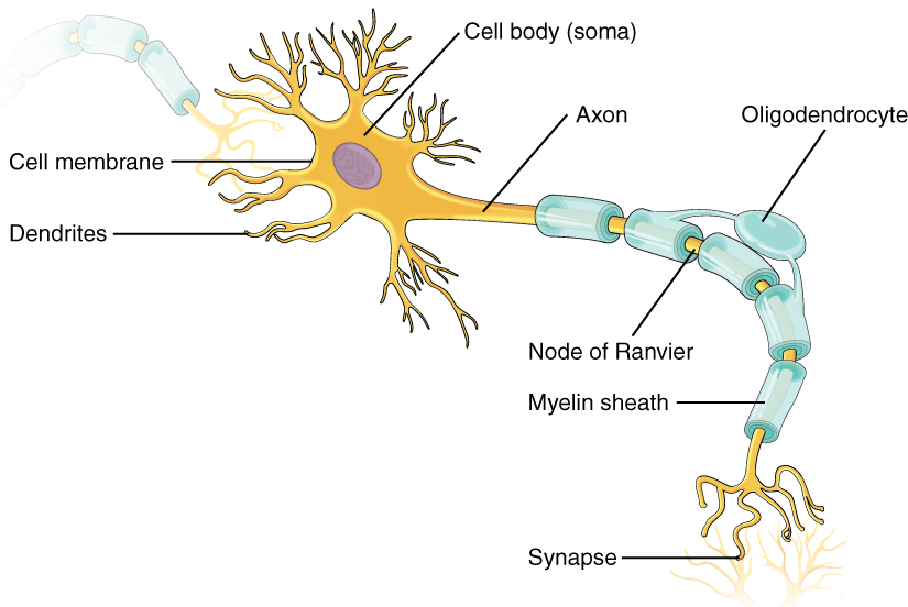
We can divide a typical neuron into three main parts: the soma, the dendrites, and the axon.[31] See the “anatomy of a neuron” section here for quick description. See Kandel et al. (2013), ch. 4-8, Lodish et al. (2008), ch. 23, and this series of videos, for detailed descriptions of basic neuron structure and function. The soma is the main body of the cell. The dendrites are extensions of the cell that branch off from the soma, and which typically receive signals from other neurons. The axon is a long, tail-like projection from the soma, which carries electrical impulses away from the cell body. The end of the axon splits into branches, the ends of which are known as axon terminals, which reach out to connect with other cells at locations called synapses. A typical synapse forms between the axon terminal of one neuron (the presynaptic neuron) and the dendrite of another (the postsynaptic neuron), with a thin zone of separation between them known as the synaptic cleft.[32] Neurons can also synapse onto blood vessels, muscle cells, neuron cell bodies, axons, and axon terminals (at least according to the medical gallery of Blausen Medical 2014), but for simplicity, I will focus on synapses between axon terminals and dendrites in what follows.
The cell as a whole is enclosed in a membrane that has various pumps that regulate the concentration of certain ions – such as sodium (Na+), potassium (K+) and chloride (Cl–) – inside it.[33]See Siegelbaum and Koester (2013a): “In addition to ion channels, nerve cells contain a second important class of proteins specialized for moving ions across cell membranes, the ion transporters or pumps. These proteins do not participate in rapid neuronal signaling but rather are important for … Continue reading This regulation creates different concentrations of these ions inside and outside the cell, resulting in a difference in the electrical potential across the membrane (the membrane potential).[34] See Siegelbaum and Koester (2013c) (p. 126-147); and the section “Where does the resting membrane potential come from?” here. The membrane also contains proteins known as ion channels, which, when open, allow certain types of ions to flow into and out of the cell.[35] See Siegelbaum and Koester (2013a) (p. 100-124), for detailed description of ion channel dynamics.
If the membrane potential in a neuron reaches a certain threshold, then a particular set of voltage-gated ion channels open to allow ions to flow into the cell, creating a temporary spike in the membrane potential (an action potential).[36] See Kandel et al. (2013) (p. 31-35); and Siegelbaum and Koester (2013b) (p. 148-171), for description. See also here. This spike travels down the axon to the axon terminals, where it causes further voltage-gated ion channels to open, allowing an influx of calcium ions into the pre-synaptic axon terminal. This calcium can trigger the release of molecules known as neurotransmitters, which are stored in sacs called vesicles in the axon terminal.[37]See Siegelbaum and Koester (2013d) (p. 184-187); Siegelbaum et al. (2013c) (p. 260-287); and description here in the section “overview of transmission at chemical synapses”). See also Lodish et al. (2008) (p. 1020). Note that action potentials do not always trigger synaptic … Continue reading
These vesicles merge with the cell membrane at the synapse, allowing the neurotransmitter they contain to diffuse across the synaptic cleft and bind to receptors on the post-synaptic neuron. These receptors can cause (directly or indirectly, depending on the type of receptor) ion channels on the post-synaptic neuron to open, thereby altering the membrane potential in that area of that cell.[38]I’ll refer to the event of a spike arriving at a synapse as a “spike through synapse.” A network of interacting neurons is sometimes called a neural circuit. A series of spikes from a single neuron is sometimes called a spike train. From Khan Academy: “we can divide the receptor … Continue reading

The expected size of the impact (excitatory or inhibitory) that a spike through a synapse will have on the post-synaptic membrane potential is often summarized via a parameter known as a synaptic weight.[40]See Open Philanthropy’s non-verbatim notes from a conversation with Prof. Shaul Druckmann: “Setting aside plasticity, most people assume that modeling the immediate impact of a pre-synaptic spike on the post-synaptic neuron is fairly simple. Specifically, you can use a single synaptic weight, … Continue reading This weight changes on various timescales, depending on the history of activity in the pre-synaptic and post-synaptic neuron, together with other factors. These changes, along with others that take place within synapses, are grouped under the term synaptic plasticity.[41] See discussion and citations in Section 2.2 for more details. Other changes also occur in neurons on various timescales, affecting the manner in which neurons respond to synaptic inputs (some of these changes are grouped under the term intrinsic plasticity).[42]Cudmore and Desai (2008): “Intrinsic plasticity is the persistent modification of a neuron’s intrinsic electrical properties by neuronal or synaptic activity. It is mediated by changes in the expression level or biophysical properties of ion channels in the membrane, and can affect such diverse … Continue reading New synapses, dendritic spines, and neurons also grow over time, and old ones die.[43] See e.g. Munno and Syed (2003), Ming and Song (2011), Grutzendler et al. (2002), Holtmaat et al. (2005).
There are also a variety of other signaling mechanisms in the brain that this basic story does not include. For example:
- Other chemical signals: Neurons can also send and receive other types of chemical signals – for example, molecules known as neuropeptides, and gases like nitric oxide – that can diffuse more broadly through the space in between cells, across cell membranes, or via the blood.[44]See Schwartz and Javitch (2013), (p. 297-301); Russo (2017); and Leng and Ludwig (2008): “Neurones use many different molecules to communicate with each other, acting in many different ways via specific receptors. Amongst these molecules are more than a hundred different peptides, expressed in … Continue reading The chemicals neurons release that influence the activity of groups of neurons (or other cells) are known as neuromodulators.[45]Burrows (1996): “A neuromodulator is a messenger released from a neuron in the central nervous system, or in the periphery, that affects groups of neurons, or effector cells that have the appropriate receptors. It may not be released at synaptic sites, often acts through second messengers and can … Continue reading
- Glial cells: Non-neuronal cells in the brain known as glia have traditionally been thought to mostly perform functions to do with maintenance of brain function, but they may be involved in task-performance as well.[46] Araque and Navarrete (2010) (p. 2375); Bullock et al. (2005), (p. 792); Mu et al. (2019); and the rest of the discussion in Section 2.3.2.
- Electrical synapses: In addition to the chemical synapses discussed above, there are also electrical synapses that allow direct, fast, and bi-directional exchange of electrical signals between neurons (and between other cells). The channels mediating this type of connection are known as gap junctions.
- Ephaptic effects: Electrical activity in neurons creates electric fields that may impact the electrical properties of neighboring neurons.[47] See e.g. Anastassiou et al. (2011) and Chang (2019), along with the other citations in Section 2.3.4.
- Other forms of axon signaling: The process of firing an action potential has traditionally been thought of as a binary decision.[48]See Bullock et al. (2005), describing the history of early neuroscience: “physiological studies established that conduction of electrical activity along the neuronal axon involved brief, all-or-nothing, propagated changes in membrane potential called action potentials. It was thus often assumed … Continue reading However, some recent evidence indicates that processes within a neuron other than “to fire or not to fire” can matter for synaptic communication.[49] See Zbili and Debanne (2019) for a review, together with the other citations in Section 2.3.5.
- Blood flow: Blood flow in the brain correlates with neural activity, which has led some to suggest that it might be playing a role in information-processing.[50]See Moore and Cao (2008): “we propose that hemodynamics also play a role in information processing through modulation of neural activity… We predict that hemodynamics alter the gain of local cortical circuits, modulating the detection and discrimination of sensory stimuli. This novel view of … Continue reading
This is not a complete list of all the possible signaling mechanisms that could in principle be operative in the brain.[51]A few others I am not discussing include: quantum dynamics (see endnote in section 1.6), the perineuronal net (see Tsien (2013) for discussion), and classical dynamics in microtubules (see Cantero et al. (2018)). I am leaving quantum dynamics aside mostly for the reasons listed in the endnote … Continue reading But these are some of the most prominent.
I want to emphasize one other meta-point about neuroscience: namely, that our current understanding of how the brain processes information is extremely limited.[52]A few representative summaries: Marcus (2015): “Neuroscience today is collection of facts, rather than ideas; what is missing is connective tissue. We know (or think we know) roughly what neurons do, and that they communicate with one another, but not what they are communicating. We know the … Continue reading This was a consistent theme in my conversations with experts, and one of my clearest take-aways from the investigation as a whole.[53] See especially Open Philanthropy’s non-verbatim notes from a conversation with Prof. Eric Jonas, Prof. Shaul Druckmann, Prof. Erik De Schutter, Prof. Konrad Kording; Prof. Eve Marder; Dr. Adam Marblestone; and Dr. Stephen Larson.
One problem is that we need better tools. For example:
- Despite advances, we can only record the spiking activity of a limited number of neurons at the same time (techniques like fMRI and EEG are much lower resolution).[54]Kleinfield et al. (2019), (p. 1005), for description of various techniques and their limitations. See also Marblestone et al. (2013): “Simultaneously measuring the activities of all neurons in a mammalian brain at millisecond resolution is a challenge beyond the limits of existing techniques in … Continue reading
- We can’t record from all of a neuron’s synapses or dendrites simultaneously, making it hard to know what patterns of overall synaptic input and dendritic activity actually occur in vivo.[55]From Open Philanthropy’s non-verbatim notes from a conversation with Prof. Erik De Schutter: “At this point, we have no way to reliably measure the input-output transformation of a neuron, where the input is defined as a specific spatio-temporal pattern of synaptic input. You can build models … Continue reading
- We also can’t stimulate all of a neuron’s synapses and/or dendrites simultaneously, making it hard to know how the cell responds to different inputs (and hence, which models can capture these responses).[56]From Open Philanthropy’s non-verbatim notes from a conversation with Prof. Erik De Schutter: “Using glutamate uncaging, you can reliably activate single dendritic spines in vitro, and you can even do this in a sequence of spines, thereby generating patterns of synaptic input. However, even … Continue reading
- Techniques for measuring many lower-level biophysical mechanisms and processes, such as possible forms of ion channel plasticity, remain very limited.[57]From Open Philanthropy’s non-verbatim notes from a conversation with Prof. Shaul Druckmann: “Technology for measuring the properties relevant to detailed biophysical modeling has improved very little in the past 20 years … Neurons can have a few dozen of some 200-300 types of ions channels, … Continue reading
- Results in model animals may not generalize to e.g. humans.[58]From Open Philanthropy’s non-verbatim notes from a conversation with Prof. Eric Jonas: “a lot of our animal models are wrong in clinically-relevant ways” (p. 5). And from Open Philanthropy’s non-verbatim notes from a conversation with Prof. E.J. Chichilnisky: “There is variability in … Continue reading
- Results obtained in vitro (that is, in a petri dish) may not generalize in vivo (that is, in a live functioning brain).[59]For example, spike-timing dependent plasticity – a form of synaptic plasticity – can be reliably elicited in vitro (see Open Philanthropy’s non-verbatim notes from a conversation with Prof. Eric Jonas (p. 3)), but Schulz argues that “Direct evidence for STDP in vivo is limited and … Continue reading
- The tasks we can give model animals like rats to perform are generally very simple, and so provide limited evidence about more complex behavior.[60]From Open Philanthropy’s non-verbatim notes from a conversation with Prof. Shaul Druckmann: “The tasks that neuroscientists tend to study in model animals are very simple. Many, for example, are some variant on a two-alternative forced choice task (e.g., teaching an animal to act differently, … Continue reading
Tools also constrain concepts. If we can’t see or manipulate something, it’s unlikely to feature in our theories.[61]From Open Philanthropy’s non-verbatim notes from a conversation with Dr. Adam Marblestone: “Neuroscience is extremely limited by available tools. For example, we have the concept of a post-synaptic potential because we can patch-clamp the post-synaptic neuron and see a change in voltage. When … Continue reading And certain models of e.g. neurons may receive scant attention simply because they are too computation-intensive to work with, or too difficult to constrain with available data.[62]From Open Philanthropy’s non-verbatim notes from a conversation with Prof. Konrad Kording: “current techniques are very bad at measuring ion channel plasticity. Neuroscientists don’t tend to focus on it for this reason” (p. 5). From Open Philanthropy’s non-verbatim notes from a … Continue reading
But tools aren’t the only problem. For example, when Jonas and Kording (2017) examined a simulated 6502 microprocessor – a system whose processing they could observe and manipulate to arbitrary degrees – using analogues of standard neuroscientific approaches, they found that “the approaches reveal interesting structure in the data but do not meaningfully describe the hierarchy of information processing in the microprocessor” (p. 1).[63]Jonas and Kording (2017): “There is a popular belief in neuroscience that we are primarily data limited…here we take a classical microprocessor as a model organism, and use our ability to perform arbitrary experiments on it to see if popular data analysis methods from neuroscience can elucidate … Continue reading And artificial neural networks that perform complex tasks are difficult (though not necessarily impossible) to interpret, despite similarly ideal experimental access.[64]See e.g. Lillicrap and Kording (2019): “…We can have a complete description of the network and its computations. And yet, neither we, nor anyone we know feels that they grasp how processing in these networks truly works. Said another way, besides gesturing to a network’s weights and … Continue reading
We also don’t know what high-level task most neural circuits are performing, especially outside of peripheral sensory/motor systems. This makes it very hard to say what models of such circuits are adequate.[65]From Open Philanthropy’s non-verbatim notes from a conversation with Prof. Eve Marder: “It’s been hard to make progress in understanding neural circuits, because in order to know what details matter, you have to know what the circuit is doing, and in most parts of the brain, we don’t know … Continue reading
It would help if we had full functional models of the nervous systems of some simple animals. But we don’t.[66]Dr. Stephen Larson suggested that one benefit of successfully simulating a simple nervous system would be that you could then bound the complexity necessary for such a simulation, and proceed with attempting to simplify it in a principled way (see Open Philanthropy’s non-verbatim notes from a … Continue reading For example, the nematode worm Caenorhabditis elegans (C. elegans) has only 302 neurons, and a map of the connections between these neurons (the connnectome) has been available since 1986.[67] See White et al. (1984). See Jabr (2012b)for some history, as well as Seung (2012): “Mapping the C. elegans nervous system took over a dozen years, though it contains only 7,000 connections” (“Introduction”). But we have yet to build a simulated C. elegans that behaves like the real worm across a wide range of contexts.[68]From Open Philanthropy’s non-verbatim notes from a conversation with Dr. Stephen Larson, who works on the OpenWorm project: “Despite its small size, we do not yet have a model that captures even 50% of the biological behavior of the C. elegans nervous system. This is partly because we’re … Continue reading
All this counsels pessimism about the robustness of FLOP/s estimates based on our current neuroscientific understanding. And it increases the relevance of where we place the burden of proof. If we start with a strong default view about the complexity of the brain’s task-performance, and then demand proof to the contrary, our standards are unlikely to be met.
Indeed, my impression is that various “defaults” in this respect play a central role in how experts approach this topic. Some take simple models that have had some success as a default, and then ask whether we have strong reason to think additional complexity necessary;[69]Example approaches in this vein include Prof. Markus Meister, see Open Philanthropy’s non-verbatim notes from a conversation with Prof. Markus Meister: “It is theoretically possible that the brain’s task-performance draws on complex chemical computations, implemented by protein circuits, … Continue reading others take the brain’s biophysical complexity as a default, and then ask if we have strong reason to think that a given type of simplification captures everything that matters.[70]From Open Philanthropy’s non-verbatim notes from a conversation with Dr. Stephen Larson: “the jury is still out on how much simplification is available, and Dr. Larson thinks that in this kind of uncertain context, you should focus on the worst-case, most conservative compute estimates as your … Continue reading
Note the distinction, though, between how we should do neuroscience, and how we should bet now about where such science will ultimately lead, assuming we had to bet. The former question is most relevant to neuroscientists; but the latter is what matters here.
Clarifying the question
Consider the set of cognitive tasks that the human brain can perform, where task performance is understood as the implementation of a specified type of relationship between a set of inputs and a set of outputs.[71]I will not attempt a definition of which tasks count as “cognitive,” but the category should be construed as excluding tasks that are intuitively particular to the brain’s biological substrate – for example, the task of implementing an input-output transformation that will serve as an … Continue reading Examples of such tasks might include:
- Reading an English-language description of a complex software problem, and, within an hour, outputting code that solves that problem.[72]See Grace et al. (2018) for discussion of a simple version of this task, which involves writing “concise, efficient, and human-readable Python code to implement simple algorithms like quicksort” (p. 19). The median estimate by the experts she surveyed for when AI systems will be able to … Continue reading
- Reading a randomly selected paper submitted to the journal Nature, and, within a week, outputting a review of the paper of quality comparable to an average peer-reviewer.[73]Depending on one’s opinions of the peer review process, perhaps it is debatable whether GPT-3 can do this as well. See here for examples. I chose both the “complex software problem” task and the “review a nature paper” task before the GPT-3 results came out, and they were selected to be … Continue reading
- Reading newly-generated Putnam Math competition problems, and, within six hours, outputting answers that would receive a perfect score by standard judging criteria.[74]It has been occasionally hypothesized that some form of quantum-level information processing is occuring in the brain (see, for example, Hu and Wu (2004), Penrose and Hameroff (2011), and Fisher (2015) for suggestions in this vein, and see Tegmark (1999) and Litt et al. (2006) for … Continue reading
Defining tasks precisely can be arduous. I’ll assume such precision is attainable, but I won’t try to attain it, since little in what follows depends on the details of the tasks in question. I’ll also drop the adjective “cognitive” in what follows.
I will also assume that sufficiently powerful computers can in principle perform these tasks (I focus solely on non-quantum computers – see endnote for discussion of quantum brain hypotheses).[75]It has been occasionally hypothesized that some form of quantum-level information processing is occuring in the brain (see, for example, Hu and Wu (2004), Penrose and Hameroff (2011), and Fisher (2015) for suggestions in this vein, and see Tegmark (1999) and Litt et al. (2006) for … Continue reading This assumption is widely shared both within the scientific community and beyond it. Some dispute it, but I won’t defend it here.[76] See Nicolesis and Circuel (2015), Lucas (1961), Dreyfus (1972) and Penrose (1994) for various forms of skepticism.
The aim of the report is to evaluate the extent to which the brain provides evidence, for some number of FLOP/s F, that for any task T that the human brain can perform, T can be performed with F.[77]Note that F does not need to be enough to match the task-performance of a “superbrain” trained and ready to perform any task that any human can perform: e.g., a brain that represents peak human performance on every task simultaneously. Einstein may do physics that requires x FLOP/s, and Toni … Continue reading As a proxy for FLOP/s numbers with this property, I will sometimes talk about the FLOP/s sufficient to run a “task-functional model,” by which I mean a computational model that replicates a generic human brain’s task-performance. Of course, some brains can do things others can’t, but I’ll assume that at the level of precision relevant to this report, human brains are roughly similar, and hence that if F FLOP/s is enough to replicate the task performance of a generic human brain, roughly F is enough to replicate any task T the human brain can perform.[78]Herculano-Houzel (2009) reports variation in neuron number within a species at around 10-50%. Reardon et al. (2018) write: “Brain size among normal humans varies as much as twofold.” Koch (2016) cites numbers ranging from 1,017 grams to 2,021 grams (though these are for post-mortem … Continue reading
The project here is related to, but distinct from, directly estimating the minimum FLOP/s sufficient to perform any task the brain can perform. Here’s an analogy. Suppose you want to build a bridge across the local river, and you’re wondering if you have enough bricks. You know of only one such bridge (the “old bridge”), so it’s natural to look there for evidence. If the old bridge is made of bricks, you could count them. If it’s made of something else, like steel, you could try to figure out how many bricks you need to do what a given amount of steel does. If successful, you’ll end up confident that e.g. 100,000 bricks is enough to build such a bridge, and hence that the minimum is less than this. But how much less is still unclear. You studied an example bridge, but you didn’t derive theoretical limits on the efficiency of bridge-building.
That said, Dr. Paul Christiano expected there to be at least some tasks such (a) the brain’s methods of performing them are close to maximally efficient, and (b) these methods use most of the brain’s resources (see endnote).[79]From Open Philanthropy’s non-verbatim notes from a conversation with Dr. Paul Christiano: “If you include a sufficiently broad range of tasks that the human brain can perform, and require similarly useful task-performance across the full range of inputs to which the brain could be exposed, it … Continue reading I don’t investigate this claim here, but if true, it would make data about the brain more directly relevant to the minimum adequate FLOP/s budget.
The project here is also distinct from estimating the FLOP/s “equivalent” to the human brain. As I discuss in the report’s appendix, I think the notion of “the FLOP/s equivalent to the brain” requires clarification: there are a variety of importantly different concepts in the vicinity.
To get a flavor of this, consider the bridge analogy again, but assume that the old bridge is made of steel. What number of bricks would be “equivalent” to the old bridge? The question seems ill-posed. It’s not that bridges can’t be built from bricks. But we need to say more about what we want to know.
I group the salient possible concepts of the “FLOP/s equivalent to the human brain” into four categories:
- FLOP/s required for task-performance, with no further constraints on how the tasks need to be performed.[80]It’s not entirely clear which concept Moravec and Kurzweil have in mind, but (1) has some support. See Moravec (1998): “How much further must this evolution proceed until our machines are powerful enough to approximate the human intellect?” (p. 52), and his reply to Anders Sandberg here: … Continue reading
- FLOP/s required for task-performance + brain-like-ness constraints – that is, constraints on the similarity between how the AI system does it, and how the brain does it.
- FLOP/s required for task-performance + findability constraints – that is, constraints on what sorts of training processes and engineering efforts would be able to create the AI system in question.
- Other analogies with human-engineered computers.
All these categories have their own problems (see section A.5 for a summary chart). The first is closest to the report’s focus, but as just noted, it’s hard (at least absent further assumptions) to estimate directly using example systems. The second faces the problem of identifying a non-arbitrary brain-like-ness constraint that picks out a unique number of FLOP/s, without becoming too much like the first. The third brings in a lot of additional questions about what sorts of systems are what sorts of findable. And the fourth, I suggest, either collapses into the first or second, or raises its own questions.
In the hopes of avoiding some of these problems, I have kept the report’s framework broad. The brain-based FLOP/s budgets I’m interested in don’t need to be uniquely “equivalent” to the brain, or as small as theoretically possible, or accommodating of any constraints on brain-like-ness or findability. They just need to be big enough, in principle, to perform the tasks in question.
A few other clarifications:
- Properties construed as consisting in something other than the implementation of a certain type of input-output relationship (for example, properties like phenomenal consciousness, moral patienthood, or continuity with a particular biological human’s personal identity – to the extent they are so construed) are not included in the definition of the type of task-performance I have in mind. Systems that replicate this type of task-performance may or may not also possess such properties, but what matters here are inputs and outputs.[81] See Sandberg and Bostrom (2008) (p. 11), for a taxonomy of possible brain-emulation success criteria. See Muehlhauser (2017) for an investigation at Open Philanthropy of consciousness and moral patienthood.
- Many tasks require more than a brain. For example, they may require something like a body, or rely partly on information-processing taking place outside the brain.[82]There is a fairly widespread discourse related to the importance of “embodiment” in AI and cognitive science more broadly, which I have not engaged with in depth. At a glance, central points seem to be: (a) that the computation a brain performs is importantly adapted to the physical environment … Continue reading In those cases, I’m interested in the FLOP/s sufficient to replicate the brain’s role.
Existing literature
(This section reviews existing literature.[83]This literature review draws from the reviews offered by Sandberg and Bostrom (2008) (p. 84-85); and Martins (2012), (p. 3-6). I have supplemented it with other estimates I encountered in my research. In order to limit its scope, I focus on direct attempts to estimate the computation sufficient … Continue reading Those interested primarily in the report’s substantive content can skip to Section 2.)
A lot of existing research is relevant to estimating the FLOP/s sufficient to run a task-functional model. But efforts in the mainstream academic literature to address this question directly are comparatively rare (a fact that this report does not alter). Many existing estimates are informal, and they often do not attempt much justification of their methods or background assumptions. The specific question they consider also varies, and their credibility varies widely.[84] The estimates that I think most worth taking seriously are generally the ones I discuss in the report itself.
Mechanistic method estimates
The most common approach assigns a unit of computation (such as a calculation, a number of bits, or a possibly brain-specific operation) to a spike through a synapse, and then estimates the rate of spikes through synapses by multiplying an estimate of the average firing rate by an estimate of the number of synapses.[85]Merkle (1989) attempts to estimate the number of spikes through synapses by estimating the energy dissipated by propagating a spike a certain distance, together with the number of synapses per unit distance, rather than counting spikes and synapses directly. He gets ~2e15 synaptic operations, … Continue reading Thus, Merkle (1989),[86] Merkle (1989): “We might count the number of synapses, guess their speed of operation, and determine synapse operations per second. There are roughly 1015 synapses operating at about 10 impulses/second, giving roughly 1016 synapse operations per second” (see “Other Estimates”). Mead (1990),[87]Mead (1990): “There are about 1016 synapses in the brain. A nerve pulse arrives at each synapse about ten times/s, on average. So in rough numbers, the brain accomplishes 1016 complex operations/s” (p. 1629). Some aspect of this estimate appears to be in error, however, as it seems to suggest … Continue reading Freitas (1996),[88] Freitas (1996): “A fair estimate is that the 1.5 kilogram organ has 1010 neurons with 103 synapses firing an average 10 times per second, which is about 1014 bits/second. Using 64-bit words like the largest supercomputers, that’s about one teraflop” (see opening section). Sarpeshkar (1997),[89]Sarpeshkar (1997): “From the numbers in the first paragraph of Section 5.6.1, we know that there are about 2.4 × 10¹⁴ synapses in each cortex of the brain. The average firing rate of cortex is about 5-10 Hz – we shall use 7.5 Hz. Assuming that each synapse is always operational and … Continue reading Bostrom (1998),[90] Bostrom (1998): “The human brain contains about 1011 neurons. Each neuron has about 5 × 10³ synapses, and signals are transmitted along these synapses at an average frequency of about 102 Hz. Each signal contains, say, 5 bits. This equals 1017 ops” (see “Hardware Requirements” section). Kurzweil (1999)),[91]Kurzweil (1999): “With an estimated average of one thousand connections between each neuron and its neighbors, we have about 100 trillion connections, each capable of a simultaneous calculation… With 100 trillion connections, each computing at 200 calculations per second, we get 20 million … Continue reading Dix (2005),[92]Dix (2005): “At a simplified level each neuron’s level of activation is determined by pulses generated at the (1000 to 10,000) synapses connected to it. Some have a positive excitatory effect [sic] some are inhibitory. A crude model simply adds the weighted sum and ‘fires’ the neuron if the … Continue reading Malickas (2007),[93]Malickas (2007): “The evaluation of the computational power of [sic] human brain [sic] very uncertain at this time. Some estimates of brain power could be based on the brain synapses number and neurons [sic] firing rate. The human brain have [sic] a 1011 neurons and each neuron has [sic] average … Continue reading and Tegmark (2017)[94]Tegmark (2017): “Multiplying together about 1011 neurons, about 104 connections per neuron and about one (100) firing per neuron each second might suggest that about 1015 FLOPS (1 petaFLOPS) suffice to simulate a human brain, but there are many poorly understood complications, including the … Continue reading are all variations on this theme.[95]Sandberg and Bostrom (2008) also cite Fiala (2007) as estimating “1014 synapses, identity coded by 48 bits plus 2 × 36 bits for pre‐and postsynaptic neuron id, 1 byte states. 10 ms update time… 256,000 terabytes/s” (p. 85), and Seitz (no date) as estimate “50-200 billion neurons, … Continue reading Their estimates range from ~1e12 to ~1e17 (though using basic different units of computation),[96] I haven’t investigated comparisons between these different units and FLOP/s (though see Sandberg and Bostrom (2008), p. 91, for some discussion of the relationship between FLOP/s and MIPS). but the variation results mainly from differences in estimated synapse count and average firing rate, rather than differences in substantive assumptions about how to make estimates of this kind.[97] As I note in Section 2.1.1.1, many of these estimates rely on average spike rates that seem to me too high. In this sense, the helpfulness of these estimates is strongly correlated: if the basic approach is wrong, none of them are a good guide.
Other estimates use a similar approach, but include more complexity. Sarpeshkar (2010) includes synaptic conductances (see discussion in section 2.1.1.2.2), learning, and firing decisions in a lower bound estimate (6e16 FLOP/s);[98]Sarpeshkar (2010): “The brain’s neuronal cells output ~1ms pulses (spikes) at an average rate of 5 Hz [55]. The 240 trillion synaptic connections [1] amongst the brain’s neurons thus lead to a computational rate of at least 1015 synaptic operations per second. A synapse implements … Continue reading Martins et al. (2012) estimate the information-processing rate of different types of neurons in different regions, for a total of ~5e16 bits/sec in the whole brain;[99] Martins et al. (2012): “These data may be combined using Eqns. (1) and (2) to yield an estimate of the synaptic-processed spike rate of Tss = (4.31 ± 0.86) × 1015 spikes/sec and the synaptic-processed bit rate of Tsb = (5.52 ± 1.13) × 1016 bits/sec for the entire human brain” (p. 14). and Kurzweil (2005) offers an upper bound estimate for a personality-level simulation of 1e19 calculations per second – an estimate that budgets 1e3 calculations per spike through synapse to capture nonlinear interactions in dendrites.[100]Kurzweil (2005): “The ‘fan out’ (number of interneuronal connections) per neuron is estimated at 103. With an estimated 1011 neurons, that’s about 1014 connections. With a reset time of five milliseconds, that comes to about 1016 synaptic transactions per second. Neuron-model simulations … Continue reading Still others attempt estimates based on protein interactions (Thagard (2002), 1e21 calculations/second);[101]Thagard (2002): “If we count the number of processors in the brain as not just the number of neurons in the brain, but the number of proteins in the brain, we get a figure of around a billion times 100 billion, or 1017. Even if it is not legitimate to count each protein as a processor all by … Continue reading microtubules (Tuszynski (2006), 1e21 FLOP/s),[102]Tuszynski (2006): “There are four c-termini states per dimer because we have two states per monomer. There could be at least four states per electron inside the tubulin dimer, as they hop between two locations. There could be at least two computational changes due to the GTP hydrolysis. Thus … Continue reading individual neurons (von Neumann (1958), 1e11 bits/second);[103]von Neumann (1958): “Thus the standard receptor would seem to accept about 14 distinct digital impressions per second, which can probably be reckoned as the same number of bits. Allowing 1010 nerve cells, assuming that each one of them is under suitable conditions essentially an (inner or outer) … Continue reading and possible computations performed by dendrites and other neural mechanisms (Dettmers (2015), 1e21 FLOP/s).[104] Dettmers (2015): “So my estimate would be 1.075×10²¹ FLOPS for the brain, the fastest computer on earth as of July 2013 has 0.58×10¹⁵ FLOPS for practical application (more about this below)” (see section “estimation of cerebellar input/output dimensions”).
A related set of estimates comes from the literature on brain simulations. Ananthanarayanan et al. (2009) estimates >1e18 FLOP/s to run a real-time human brain simulation;[105] See Ananthanarayanan et al. (2009), Figure 8 (p. 10). Greenemeier (2009) cites IBM’s Dharmendra Modha (one of the authors on the paper) as estimating that a computer comparable to the human brain would need to perform 4e16 operations per second, but I’m not sure his methodology. Waldrop (2012) cites Henry Markram as estimating 1e18 FLOP/s to run a very detailed simulation;[106]Waldrop (2012): “The computer power required to run such a grand unified theory of the brain would be roughly an exaflop, or 1018 operations per second — hopeless in the 1990s. But Markram was undaunted: available computer power doubles roughly every 18 months, which meant that exascale … Continue reading Markram, in a 2018 video (18:28), estimates that you’d need ~4e29 FLOP/s to run a “real-time molecular simulation of the human brain”;[107] He also discusses a possible lower estimate around 19:43, but the video is too blurry for me to read the numbers. and Eugene Izhikevich estimates that a real-time brain simulation would require ~1e6 processors running at 384 GHz.[108] See here. See also Izhikevich and Edelman (2007).
Sandberg and Bostrom (2008) also estimate the FLOP/s requirements for brain emulations at different levels of detail. Their estimates range from 1e15 FLOP/s for an “analog network population model,” to 1e43 FLOP/s for emulating the “stochastic behavior of single molecules.”[109]See Sandberg and Bostrom (2008) (p. 80-81). My impression is that these estimates were very rough, and their 1e18 estimate for a spiking neural network seems inconsistent with the estimate methodology they use elsewhere in the chart, since 1e15 entities × 10 FLOPs per entity × 1e3 time-steps … Continue reading They report that in an informal poll of attendees at a workshop on whole brain emulation, the consensus appeared to be that the required level of resolution would fall between “Spiking neural network” (1e18 FLOP/s), and “Metabolome” (1e25 FLOP/s).[110] Strong selection effects were like at work in determining who was present at the workshop.
Despite their differences, I group all of these estimates under the broad heading of the “mechanistic method,” as all of them attempt to identify task-relevant causal structure in the brain’s biological mechanisms, and quantify it in some kind of computational unit.
Functional method estimates
A different class of estimates focus on the FLOP/s sufficient to replicate the function of some portion of the brain, and then attempt to scale up to an estimate for the brain as a whole (the “functional method”). Moravec (1988), for example, estimates the computation required to do what the retina does (1e9 calculations/second) and then scales up (1e14 calc/s).[111] See Moravec (1988), Chapter 2 (p. 51-74). See also Moravec (1988), Moravec (2008). I discuss this estimate in detail in Section 3.1. Merkle (1989) performs a similar retina-based calculation and gets 1e12-1e14 ops/sec.[112] Kurzweil (2005) also cites Zaghloul and Boahen (2006) as an example of replicating retinal functionality, but does not attempt a quantitative estimate using it (endnote 41, p. 532).
Kurzweil (2005) offers a functional method estimate (1e14 calcs/s) based on work by Lloyd Watts on sound localization,[113]Kurzweil (2005): “Another estimate comes from the work of Lloyd Watts and his colleagues on creating functional simulations of regions of the human auditory system, which I discuss further in chapter 4… Watts’s own group has created functionally equivalent re-creations of these brain regions … Continue reading another (1e15 calcs/s) based on an cerebellar simulation at the University of Texas;[114]Kurzweil (2005): “Yet another estimate comes from a simulation at the University of Texas that represents the functionality of a cerebellum region containing 104 neurons; this required about 108 cps, or about 104 cps per neuron. Extrapolating this over an estimated 1011 neurons results in a … Continue reading and a third (1e14 calcs/s), in his 2012 book, based on the FLOP/s he estimates is required to emulate what he calls a “pattern recognizer” in the neocortex.[115]Kurzweil (2012): “emulating one cycle in a single pattern recognizer in the biological brain’s neocortex would require about 3,000 calculations. Most simulations run at a fraction of this estimate. With the brain running at about 102 (100) cycles per second, that comes to 3 × 10⁵ (300,000) … Continue readingDrexler (2019) uses the FLOP/s required for various deep learning systems (specifically: Google’s Inception architecture, Deep Speech 2, and Google’s neural machine translation model) to generate various estimates he takes to suggest that 1e15 FLOP/s is sufficient to match the brain’s functional capacity.[116]Drexler (2019): “In light of the above comparisons, all of which yield values of RPFLOP in the 10 to 1000 range, it seems likely that 1 PFLOP/s machines equal or exceed the human brain in raw computation capacity. To draw the opposite conclusion would require that the equivalents of a wide range … Continue reading
Limit method estimates
Sandberg (2016) uses Landauer’s principle to generate an upper bound of ~2e22 irreversible operations per second in the brain – a methodology I consider in more detail in Section 4.[117] Sandberg (2016): “20 W divided by 1.3 × 10⁻²¹ J (the Landauer limit at body temperature) suggests a limit of no more than 1.6·1022 irreversible operations per second” (p. 5). De Castro (2013) estimates a similar limit, also from Landauer’s principle, on perceptual operations performed by the parts of the brain involved in rapid, automatic inference (1e23 operations per second).[118]De Castro (2013): “If system 1 is considered to be a powerful computer operating at maximum Landauer efficiency—i.e., at a minimum energy cost equal to kBT ln(2)—that works at an average brain temperature, the number of perceptual operations per second that it could perform is on the order of … Continue reading I have yet to encounter other attempts to bound the brain’s overall computation via Landauer’s principle,[119] Though there is some discussion of it on Metaculus. though many papers discuss related issues in the brain and in biological systems more broadly.[120]For example, Laughlin et al. (1998) estimate that “synapses and cells are using 105 to 108 times more energy than the thermodynamic minimum” (the minimum they have in mind is on the order of a kT per bit “observed”); and Levy et al. (2014) argue that once the costs of communication … Continue reading
Communication method estimates
AI Impacts estimates the communication capacity of the brain (measured as “traversed edges per second” or TEPS), then combines this with an observed ratio of TEPS to FLOP/s in some human-engineered computers, to arrive an estimate of brain FLOP/s (~1e16-3e17 FLOP/s).[121]AI Impacts: “Among a small number of computers we compared4, FLOPS and TEPS seem to vary proportionally, at a rate of around 1.7 GTEPS/TFLOP. We also estimate that the human brain performs around 0.18 – 6.4 × 10¹⁴ TEPS. Thus if the FLOPS:TEPS ratio in brains is similar to that in computers, … Continue reading I discuss methods in this broad category – what I call, the “communication method” – in Section 5.
Let’s turn now to evaluating the methods themselves. Rather than looking at all possible ways of applying them, my discussion will focus on what seem to me like the most plausible approaches I’m aware of, and the most important arguments/objections.
The mechanistic method
The first method I’ll be discussing – the “mechanistic method” – attempts to estimate the computation required to model the brain’s biological mechanisms at a level of detail adequate to replicate task performance.
Simulating the brain in extreme detail would require enormous amounts of computational power.[122]See e.g. the rough estimates from Sandberg and Bostrom (2008) (p. 80-81), to the effect that emulating the states of the protein complexes in the brain would require 1e27 FLOP/s, and that emulating the stochastic behavior of single molecules in the brain would require 1e43 FLOP/s. Henry Markham, … Continue reading Which details would need to be included in a computational model, and which, if any, could be left out or summarized?
The approach I’ll pursue focuses on signaling between cells. Here, the idea is that for a process occurring in a cell to matter to task-performance, it needs to affect the type of signals (e.g. neurotransmitters, neuromodulators, electrical signals at gap junctions, etc.) that cell sends to other cells.[123]I first encountered the idea that the computational relevance of processes within the neuron are bottlenecked by intercellular signaling via one of our technical advisors, Dr. Dario Amodei. See also Open Philanthropy’s non-verbatim notes from a conversation with Prof. Dong Song: “Prof. Song … Continue reading Hence, a model of that cell that replicates its signaling behavior (that is, the process of receiving signals, “deciding” what signals to send out, and sending them) would replicate the cell’s role in task-performance, even if it leaves out or summarizes many other processes occuring in the cell. Do that for all the cells in the brain involved in task-performance, and you’ve got a task-functional model.
I’ll divide the signaling processes that might need to be modeled into three categories:
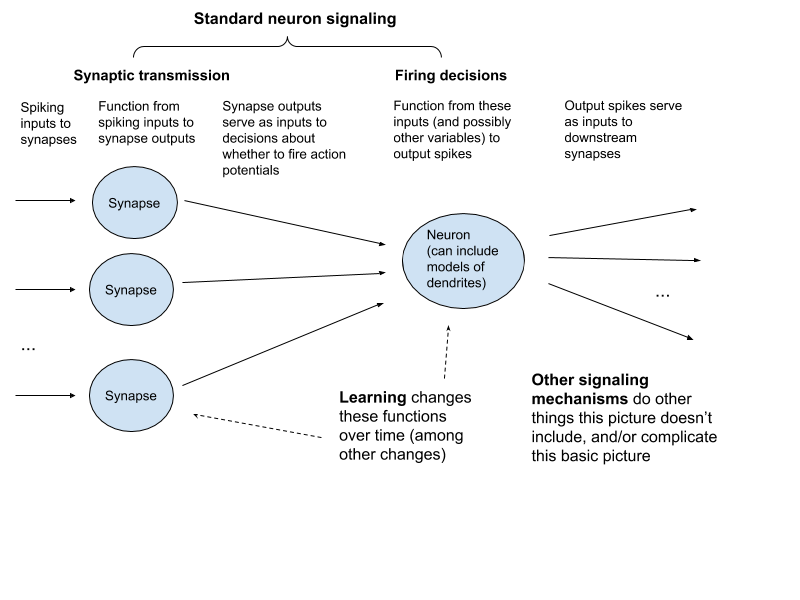
- Standard neuron signaling.[124] “Standard” here indicates “the type of neuron signaling people tend to focus on.” Whether it is the signaling method that the brain relies on most heavily is a more substantive question. I’ll divide this into two parts:
- Synaptic transmission. The signaling process that occurs at a chemical synapse as a result of a spike.
- Firing decisions. The processes that cause a neuron to spike or not spike, depending on input from chemical synapses and other variables.
- Learning. Processes involved in learning and memory formation (e.g., synaptic plasticity, intrinsic plasticity, and growth/death of cells and synapses), where not covered by (1).
- Other signaling mechanisms. Any other signaling mechanisms (neuromodulation, electrical synapses, ephaptic effects, glial signaling, etc.) not covered by (1) or (2).
As a first-pass framework, we can think of synaptic transmission as a function from spiking inputs at synapses to some sort of output impact on the post-synaptic neuron; and of firing decisions as (possibly quite complex) functions that take these impacts as inputs, and then produce spiking outputs – outputs which themselves serve as inputs to downstream synaptic transmission. Learning changes these functions over time (though it can involve other changes as well, like growing new neurons and synapses). Other signaling mechanisms do other things, and/or complicate this basic picture.
This isn’t an ideal carving, but hopefully it’s helpful regardless.[125]In particular, the categories plausibly overlap: much of the standard neuron signaling in the brain may be in the service of what would generally be folk-theoretically understood as “learning” (see Open Philanthropy’s non-verbatim notes from a conversation with Dr. Adam Marblestone: “it … Continue reading Here’s the mechanistic method formula that results:
Total FLOP/s = FLOP/s for standard neuron signaling +
FLOP/s for learning +
FLOP/s for other signaling mechanisms
I’m particularly interested in the following argument:
- You can capture standard neuron signaling and learning with somewhere between ~1e13-1e17 FLOP/s overall.
- This is the bulk of the FLOP/s burden (other processes may be important to task-performance, but they won’t require comparable FLOP/s to capture).
I’ll discuss why one might find (I) and (II) plausible in what follows. I don’t think it at all clear that these claims are true, but they seem plausible to me, partly on the merits of various arguments I’ll discuss, and partly because some of the experts I engaged with were sympathetic (others were less so). I also discuss some ways this range could be too high, and too low.
Standard neuron signaling
Here is the sub-formula for standard neuron signaling:
FLOP/s for standard neuron signaling = FLOP/s for synaptic transmission + FLOP/s for firing decisions
I’ll budget for each in turn.
Synaptic transmission
Let’s start with synaptic transmission. This occurs as a result of spikes through synapses, so I’ll base this budget on spikes through synapses per second × FLOPs per spike through synapse (I discuss some assumptions this involves below).
Spikes through synapses per second
How many spikes through synapses happen per second?
As noted above, the human brain has roughly 100 billion neurons.[126]Azevedo et al. (2009): “We find that the adult male human brain contains on average 86.1 ± 8.1 billion NeuN-positive cells (“neurons”) and 84.6 ± 9.8 billion NeuN-negative (“nonneuronal”) cells” (532). My understanding is that the best available method of counting neurons is … Continue reading Synapse count appears to be more uncertain,[127] See e.g. Pakkenberg et al. (2002): “Synapses have a diameter of 200–500 nm and can only be seen by electron microscopy. The primary problem in assessing the number of synapses in human brains is their lack of resistance to the decay starting shortly after death” (p. 98). but most estimates I’ve seen fall in the range of an average of 1,000-10,000 synapses per neuron, and between 1e14 and 1e15 overall.[128]Kandel et al. (2013): “An average neuron forms and receives 1,000 to 10,000 synaptic connections. Thus 1014 to 1015 synaptic connections are formed in the brain” (p. 175). Henry Markram uses 1e15 total synapses in this video (18:31); AI Impacts suggests 1.8-3.2e14. A number of synapse … Continue reading
How many spikes arrive at a given synapse per second, on average?
- Maximum neuron firing rates can exceed 100 Hz,[129]Wang et al. (2016): “By recording in human, monkey, and mouse neocortical slices, we revealed that FS neurons in human association cortices (mostly temporal) could generate APs at a maximal mean frequency (Fmean) of 338 Hz and a maximal instantaneous frequency (Finst) of 453 Hz, and they increase … Continue reading but in vivo recordings suggest that neurons usually fire at lower rates – between 0.01 and 10 Hz.[130]Barth and Poulet (2012) (p. 4-5), list a large number firing rates overserved in rat neurons, almost all of which appear to be below 10 Hz. Buzaki and Mizuseki (2014): “Recent quantifications of firing patterns of cortical pyramidal neurons in the intact brain have shown that the mean … Continue reading
- Experts I engaged with tended to use average firing rates of 1-10 Hz.[131]Anthony Zador used an average rate of 1 Hz (see Open Philanthropy’s non-verbatim notes from a conversation with Prof. Anthony Zador, p. 4). Konrad Kording suggested that neurons run at roughly 10 Hz (see Open Philanthropy’s non-verbatim notes from a conversation with Prof. Konrad Kording). … Continue reading
- Energy costs limit spiking. Lennie (2003), for example, uses energy costs to estimate a 0.16 Hz average in the cortex, and 0.94 Hz “using parameters that all tend to underestimate the cost of spikes.”[132] See p. 494-495. He also estimates that “to sustain an average rate of 1.8 spikes/s/neuron would use more energy than is normally consumed by the whole brain” (13 Hz would require more than the whole body).[133] P. 495.
- Existing recording methods may bias towards active cells.[134]Barth and Poulet (2012): “accumulating experimental evidence, using non-selective methods to assess the activity of identified, individual neurons, indicates that traditional extracellular recordings may have been strongly biased by selection of the most active cells” (p. 1). Buzaki and … Continue reading Shoham et al. (2005), for example, suggests that recordings may overlook large numbers of “silent” neurons that fire infrequently (on one estimate for the cat primary visual cortex, >90% of neurons may qualify as “silent”).[135]Shoham et al. (2005): “To summarize, the existence of large populations of silent neurons has been suggested recently by experimental evidence from diverse systems. Only some regions and neuron types show this phenomenon: as counterexamples, interneurons and cerebellar Purkinje cells are active … Continue reading
Synthesizing evidence from a number of sources, AI Impacts offers a best guess average of 0.1-2 Hz. This sounds reasonable to me (I give most weight to the metabolic estimates). I’ll use 0.1-1 Hz, partly because Lennie (2003) treats 0.94 Hz as an overestimate, and partly because I’m mostly sticking with order-of-magnitude level precision. This suggests an overall range of ~1e13-1e15 spikes through synapses per second (1e14-1e15 synapses × 0.1-1 spikes per second).[136]It’s also possible that the metabolic considerations could be used as evidence for the combinations of synapse count and average spiking rate that would be compatible with the brain’s energy budget. For example, it’s possible that 10,000 synapses per neuron is incompatible with higher average … Continue reading
Note that many of the mechanistic method estimates reviewed in 1.6.1 assume a higher average spiking rate, often in the range of 100 Hz.[137]Examples include: Bostrom (1998): “signals are transmitted along these synapses at an average frequency of about 102 Hz” (“Hardware requirements”); Mead (1990): “A nerve pulse arrives at each synapses about ten times/s, on average” (p. 1629); Merkle (1989): “There are roughly … Continue reading For the reasons listed above, I think 100 Hz too high. ~10 Hz seems more possible (though it requires Lennie (2003) to be off by 1-2 orders of magnitude, and my best guess is lower): in that case, we’d add an orders of magnitude to the high-end estimates below.
FLOPs per spike through synapse
How many FLOPs do we need to capture what matters about the signaling that occurs when a spike arrives at a synapse?
A simple model
A simple answer is: one FLOP. Why might one think this?
One argument is that in the context of standard neuron signaling (setting aside learning), what matters about a spike through a synapse is that it increases or decreases the post-synaptic membrane potential by a certain amount, corresponding to the synaptic weight. This could be modeled as a single addition operation (e.g., add the synaptic weight to the post-synaptic membrane potential). That is, one FLOP (of some precision, see below).[138]This model of synaptic transmission was suggested by our technical advisor, Dr. Dario Amodei. See also Open Philanthropy’s non-verbatim notes from a conversation with Prof. Shaul Druckmann: “Setting aside plasticity, most people assume that modeling the immediate impact of a pre-synaptic spike … Continue reading
We can add several complications without changing this picture much:[139] The bullet points below were inspired by comments from Dr. Dario Amodei as well.
- Some estimates treat a spike through a synapse as multiplication by a synaptic weight. But spikes are binary, so in a framework based on individual spikes, you’re really only “multiplying” the synaptic weight by 0 or 1 (e.g., if the neuron spikes, then multiply the weight by 1, and add it to the post-synaptic membrane potential; otherwise, multiply it by 0, and add the result – 0 – to the post-synaptic membrane potential).
- In artificial neural networks, input neuron activations are sometimes analogized to non-binary spike rates (e.g., average numbers of spikes over some time interval), which are multiplied by synaptic weights and then summed.[140] See Matt Botvinick’s comments on this podcast: “The activity of units in a deep learning system is broadly analogous to the spike rate of a neuron” (see 57.20 here). This would be two FLOPs (or one Multiply-Accumulate). But since such rates take multiple spikes to encode, this analogy plausibly suggests less than two FLOPs per spike through synapse.
How precise do these FLOPs need to be?[141] Precision, here, refers to number of bits used to represent the floating point numbers in question. That depends on the number of distinguishable synaptic weights/membrane potentials. Here are some relevant estimates:
- Koch (1999) suggests “between 6 and 7 bits of resolution” for variables like neuron membrane potential.[142]Koch (1999): “It is doubtful whether the effective resolution, that is, the ratio of minimal change in any one variable, such as Vm or [Ca2+]i, relative to the noise amplitude associated with this variable, exceeds a factor of 100. Functionally, this corresponds to between 6 and 7 bits of … Continue reading
- Bartol et al. (2015) suggest a minimum of “4.7 bits of information at each synapse” (they don’t estimate a maximum).[143]See Bartol et al. (2015) (abstract): “Signal detection theory holds that at a Signal-to-Noise Ratio (SNR) of 1, a common detection threshold used in psychophysical experiments, an ideal observer can correctly detect whether a signal is higher or lower than some threshold 69% of the time (Green … Continue reading
- Sandberg and Bostrom (2008) cite evidence for ~1 bit, 3-5 bits, and 0.25 bits stored at each synapse.[144]Sandberg and Bostrom (2008): “Assumption on the order of one bit of information per synapse has some support on theoretical grounds. Models of associative neural networks have an information storage capacity slightly under 1 bit per synapse depending on what kind of information is encoded (Nadal … Continue reading
- Zador (2019) suggests “a few” bits/synapse to specify graded synaptic strengths.[145] Zador (2019): “a few extra bits/synapse would be required to specify graded synaptic strengths. But because of synaptic noise and for other reasons, synaptic strength may not be specified very precisely” (p. 5).
- Lahiri and Ganguli (2013) suggest that the number of distinguishable synaptic strengths can be “as small as two”[146]Lahiri and Ganguli (2013): “recent experimental work has shown that many synapses are more digital than analog; they cannot robustly assume an infinite continuum of analog values, but rather can only take on a finite number of distinguishable strengths, a number than can be as small as two … Continue reading (though they cite Enoki et al. (2009) as indicating greater precision).[147] Enoki et al. (2009): “The results demonstrate that individual Schaffer collateral synapses on CA1 pyramidal neurons behave in an incremental rather than binary fashion, sustaining graded and bidirectional long-term plasticity” (“summary”).
A standard FLOP is 32 bits, and half-precision is 16 – well in excess of these estimates. Some hardware uses even lower-precision operations, which may come closer. I’d guess that 8 bits would be adequate.
If we assume 1 (8-bit) FLOP per spike through synapse, we get an overall estimate of 1e13-1e15 (8-bit) FLOP/s for synaptic transmission. I won’t continue to specify the precision I have in mind in what follows.
Here are a few complications this simple model leaves out.
Stochasticity
Real chemical synaptic transmission is stochastic. Each vesicle of neurotransmitter has a certain probability of release, conditional on a spike arriving at the synapse, resulting in variation in synaptic efficacy across trials.[148]Siegelbaum et al. (2013c): “The mean probability of transmitter release from a single active zone also varies widely among different presynaptic terminals, from less than 0.1 (that is, a 10% chance that a presynaptic action potential will trigger release of a vesicle) to greater than 0.9” … … Continue reading This isn’t necessarily a design defect. Noise in the brain may have benefits,[149] See e.g. McDonnel and Ward (2011), Jonas (2014, unpublished), and Faisel et al. (2008) (p. 3) for discussion of the benefits of noise. and we know that the brain can make synapses reliable.[150]As Siegelbaum et al. (2013c) note, “in synaptic connections where a low probability of release is deleterious for function, this limitation is overcome by simply having many active zones [that is, neurotransmitter release sites] in one synapse” (p. 271). The fact that the brain can choose to … Continue reading
Would capturing the contribution of this stochasticity to task performance require many extra FLOP/s, relative to a deterministic model? My guess is no.
- The relevant probability distribution (a binomial distribution, according to Siegelbaum et al. (2013c), (p. 270)), appears to be fairly simple, and Dr. Paul Christiano, one of our technical advisors, thought that sampling from an approximation of such a distribution would be cheap.[151]From Open Philanthropy’s non-verbatim notes from a conversation with Dr. Paul Christiano: “One way of modeling synaptic stochasticity is by assigning a fixed release probability to each synaptic vesicle, conditional on presynaptic activity. Dr. Christiano does not think that modeling spikes … Continue reading
- My background impression is that in designing systems for processing information, adding noise is easy; limiting noise is hard (though this doesn’t translate directly into a FLOPs number).
- Despite the possible benefits of noise, my guess is that the brain’s widespread use of stochastic synapses has a lot to do with resource constraints (more reliable synapses require more neurotransmitter release sites).[152] See Seigelbaum et al. (2013) quotes above. From Open Philanthropy’s non-verbatim notes from a conversation with Prof. Erik De Schutter: “Some hypothesize that it’s about energy efficiency, but there is no proof of this.” (p. 3).
- Many neural network models don’t include this stochasticity.[153]From Open Philanthropy’s non-verbatim notes from a conversation with Prof. Erik De Schutter: “[synaptic stochasticity] is almost never included in neural network models” (p. 3). From Open Philanthropy’s non-verbatim notes from a conversation with Prof. Chris Eliasmith: ‘Pretty much … Continue reading
That said, one expert I spoke with (Prof. Erik De Schutter) thought it an open question whether the brain manipulates synaptic stochasticity in computationally complex ways.[154]From Open Philanthropy’s non-verbatim notes from a conversation with Prof. Erik De Schutter: “It’s an open question whether you could capture this stochasticity by drawing from a relatively simple distribution, or whether the brain manipulates synaptic stochasticity in more computationally … Continue reading
Synaptic conductances
The ease with which ions can flow into the post-synaptic cell at a given synapse (also known as the synaptic conductance) changes over time as the ion channels activated by synaptic transmission open and close.[155] This change can be modeled in different ways (for example, as an exponential decay, or as a difference of exponentials), and different post-synaptic receptors exhibit different behaviors. See Dayan and Abbott (2001) (p. 182), Figure 5.15, and the pictures of different models here. The simple “addition” model above doesn’t include this – rather, it summarizes the impact of a spike through synapse as a single, instantaneous increase or decrease to post-synaptic membrane potential.
Sarpeshkar (2010), however, appears to treat the temporal dynamics of synaptic conductances as central to the computational function of synapses.[156]Sarpeshkar (2010): “Synapses are effectively spike-dependent electrochemical gm generators [my understanding is that “gm” stands for conductance]. They convert the input digital spike impulse arriving from a presynaptic transmitting neuronal axon into an exponential analog impulse-response … Continue reading He assumes, as a lower bound, that “the 20 ms second-order filter response due to each synapse is 40 FLOPs,” and that such operations occur on every spike.[157]Sarpeshkar (2010): “A synapse implements multiplication and filtering operations on every spike and sophisticated learning operations over multiple spikes. If we assume that synaptic multiplication is at least one floating-point operation (FLOP), the 20 ms second-order filter impulse response due … Continue reading
I’m not sure exactly what Sarpeshkar (2010) has in mind here, but it seems plausible to me that the temporal dynamics of a neuron’s synaptic conductances can influence membrane potential, and hence spike timing, in task-relevant ways.[158]I’m partly influenced here by comments from Dr. Adam Marblestone, see Open Philanthropy’s non-verbatim notes from a conversation with Dr. Adam Marblestone: “If you neglect this temporal shape, you’ll get the wrong output: it matters that incoming spikes coincide and add up properly” (p. … Continue readingOne expert also emphasized the complications to neuron behavior introduced by the conductance created by a particular type of post-synaptic receptor called an NMDA-receptor – conductances that Beniaguev et al. (2020) suggest may substantially increase the complexity of a neuron’s I/O (see discussion in Section 2.1.1.2).[159]See Open Philanthropy’s non-verbatim notes from a conversation with Prof. Shaul Druckmann: “the long time-constant of NMDA receptors increases the complexity of the neuron’s input-output transformation” (p. 3). Beniaguev et al. (2020): “Detailed studies of synaptic integration in … Continue reading That said, two experts thought it likely that synaptic conductances could either be summarized fairly easily or left out entirely.[160]From Open Philanthropy’s non-verbatim notes from a conversation with Prof. Anthony Zador: “He does not think that … we need to include the details of synaptic conductances in our models” (p. 1). From Open Philanthropy’s non-verbatim notes from a conversation with Dr. Adam Marblestone: … Continue reading
Sparse FLOPs and time-steps per synapse
Estimates based on spikes through synapses assume that you don’t need to budget any FLOPs for when a synapse doesn’t receive a spike, but could have. Call this the “sparse FLOPs assumption.”[161] My discussion of this assumption is inspired by some comments from Dr. Dario Amodei. In current neural network implementations, the analogous situation (e.g., artificial neuron activations of 0) creates inefficiencies, which some new hardware designs aim to avoid.[162]See, for example, the recent Cerebras whitepaper: “Multiplying by zero is a waste—a waste of silicon, power, and time, all while creating no new information. In deep learning, the data are often very sparse. Half to nearly all the elements in the vectors and matrices that are to be multiplied … Continue reading But this seems more like an engineering challenge than a fundamental feature of the brain’s task-performance.
Note, though, that for some types of brain simulation, budgets would be based on time-steps per synapse instead, regardless of what is actually happening at synapse over that time. Thus, for a simulation of a 1e14-1e15 synapses run at 1 ms resolution (1000 timesteps per second), you’d get 1e17-1e18 timesteps per synapse – a number that would then be multiplied by your FLOPs budget per time-step at each synapse; and smaller time-steps would yield higher numbers. Not all brain simulations do this (see, e.g., Ananthanarayanan et al. (2009), who simulate time-steps at neurons, but events at synapse),[163]Ananthanarayanan et al. (2009): “The basic algorithm of our cortical simulator C2 [2] is that neurons are simulated in a clock-driven fashion whereas synapses are simulated in an event-driven fashion. For every neuron, at every simulation time step (say 1 ms), we update the state of each neuron, … Continue reading but various experts use it as a default methodology.[164] See e.g. Sandberg and Bostrom (2008) (p. 80-81); and Henry Markram, in a 2018 video (18:28).
Going forward, I’ll assume that on simple models of synaptic transmission where the synaptic weight is not changing during time-steps without spikes, we don’t need to budget any FLOPs for those time-steps (the budgets for different forms of synaptic plasticity are different story, and will be covered in the learning section). If this is wrong, though, it could increase budgets by a few orders of magnitude (see Section 2.4.1).
Others
There are likely many other candidate complications that the simple model discussed above does not include. There is intricate molecular machinery located at synapses, much of which is still not well-understood. Some of this may play a role in synaptic plasticity (see Section 2.2 below), or just in maintaining a single synaptic weight (itself a substantive task), but some may be relevant to standard neuron signaling as well.[165]From Open Philanthropy’s non-verbatim notes from a conversation with Prof. Blake Richards: “Some neuroscientists are interested in the possibility that a lot of computation is occurring via molecular processes in the brain. For example, very complex interactions could be occurring in a … Continue reading
Higher-end estimate
I’ll use 100 FLOPs per spike through synapse as a higher-end FLOP/s budget for synaptic transmission. This would at least cover Sarpeshkar’s 40 FLOP estimate, and provide some cushion for other things I might be missing, including some more complex manipulations of synaptic stochasticity.
With 1 FLOP per spike through synapse as a low-end, and 100 FLOPs as a high end, we get 1e13-1e17 FLOP/s overall. Firing rate models might suggest lower numbers; other complexities and unknowns, along with estimates based on time-steps rather than spikes, higher numbers.
Firing decisions
The other component of standard neuron signaling is firing decisions, understood as mappings from synaptic inputs to spiking outputs.
One might initially think these likely irrelevant: there are 3-4 orders of magnitude more synapses than neurons, so one might expect events at synapses to dominate the FLOP/s burden.[166]From Open Philanthropy’s non-verbatim notes from a conversation with Prof. Barak Pearlmutter: “Prof. Pearlmutter thought that the compute for firing decisions would be “in the noise” relative to compute for spikes through synapses, because there are so many fewer neurons than synapses” … Continue reading But as just noted, we’re counting FLOPs at synapses based on spikes, not time-steps. Depending on the temporal-resolution we use (this varies across models), the number of time-steps per second (often ≥1000) plausibly exceeds the average firing rate (~0.1-1 Hz) by 3-4 orders of magnitude as well. Thus, if we need to compute firing decisions every time-step, or just generally more frequently than the average firing rate, this could make up for the difference between neuron and synapse count (I discuss this more in Section 2.1.2.5). And firing decisions could be more complex than synaptic transmission for other reasons as well.
Neuroscientists implement firing decisions using neuron models that can vary enormously in their complexity and biological realism. Herz et al. (2006) group these models into five rough categories:[167] See Fig. 1. (p. 80).
- Detailed compartmental models. These attempt detailed reconstruction of a neuron’s physical structure and the electrical properties of its dendritic tree. This tree is modeled using many different “compartments” that can each have different membrane potentials.
- Reduced compartmental models. These include fewer distinct compartments, but still more than one.
- Single compartment models. These ignore the spatial structure of the neuron entirely and focus on the impact of input currents on the membrane potential in a single compartment.
- The Hodgkin-Huxley model, a classic model in neuroscience, is a paradigm example of a single compartment model. It models different ionic conductances in the neuron using a series of differential equations. According to Izhikevich (2004), it requires ~120 FLOPs per 0.1 ms of simulation – ~1e6 FLOP/s overall.[168] See figure 2.
- My understanding is that “integrate-and-fire”-type models – another classic neuron model, but much more simplified – would also fall into this category. Izhikevich (2004) suggests that these require ~5-13 FLOPs per ms per cell, 5000-13,000 FLOP/s overall.[169] See figure 2. Integrate and fire models are roughly 5-15 FLOPs per ms: Hodgkin-Huxley is 1200.
- Cascade models. These models abstract away from ionic conductances, and instead attempt to model a neuron’s input-output mapping using a series of higher-level linear and non-linear mathematical operations, together with sources of noise. The “neurons” used in contemporary deep learning can be seen as variants of models in this category.[170] One expert I spoke to said this, though the comment didn’t end up in the conversation notes. These cascade models can also incorporate operations meant to capture transformations of synaptic inputs that occur in dendrites.[171] See Fig. 3. (p. 83), in Herz et al. (2006). The two-layer cascade model they discuss resembles the one suggested by Poirazi et al. (2003). See Section 2.1.2.2 for more discussion of dendritic computation in particular.
- Black box models. These neglect biological mechanisms altogether.
Prof. Erik De Schutter also mentioned that greater computing power has made even more biophysically realistic models available.[172]From Open Philanthropy’s non-verbatim notes from a conversation with Prof. Erik De Schutter: “Old multi-compartmental models, based on cable theory, described voltage in one dimension, and the typical resolution was on the order of tens of microns per compartment. That is adequate for modeling … Continue reading And models can in principle be arbitrarily detailed.
Which of these models (if any) would be adequate to capture what matters about firing decisions? I’ll consider four categories of evidence: the predictive success of different neuron models; some specific arguments about the computational power of dendrites; a collection of other considerations; and expert opinion/practice.
Predicting neuron behavior
Let’s first look at the success different models have had in predicting neuron spike patterns.
Standards of accuracy
How accurate do these predictions need to be? The question is still open.
In particular, debate in neuroscience continues about whether and when to focus on spike rates (e.g., the average number of spikes over a given period), vs. the timings of individual spikes.[173]From a review article by Brette (2015): “Do individual spikes matter or can neural computation be essentially described in terms of rates, with spikes physically instantiating this description? This contentious question has generated considerable debate in neuroscience, and is still unsettled” … Continue reading
- Many results in neuroscience focus on rates,[174]Koch (1999) describes a standard procedure: “In a typical physiological experiment, the same stimulus is presented multiple times to a neuron and its response is recorded (Fig. 14.1). One immediately notices that the detailed response of the cell changes from trial to trial….Given the … Continue reading as do certain neural prostheses.[175]See e.g. Hochberg (2012): “Raw neural signals for each channel were sampled at 30 kHz and fed through custom Simulink (Mathworks Inc., Natick, MA) software in 100 ms bins (S3) or 20 ms bins (T2) to extract threshold crossing rates; these threshold crossing rates were used as the neural features … Continue reading
- In some contexts, it’s fairly clear that spike timings can be temporally precise.[176]See e.g. Weiss et al. (2018): “many sensory systems use millisecond or even sub-millisecond precise spike timing across sensory neurons to rapidly encode stimulus features (e.g., visual patterns in salamanders [Gollisch and Meister (2008)], direction of sound in barn owls [Carr and Konishi … Continue reading
- One common argument for rates appeals to variability in a neuron’s response to repeated exposure to the same stimulus.[177]Brette (2015): “Perhaps the most used argument against spike-based theories is the fact that spike trains in vivo are variable both temporally and over trials (Shadlen and Newsome (1998)), and yet this might well be the least relevant argument. This assertion is what philosophers call a … Continue reading My impression is that this argument is not straightforward to make rigorous, but it seems generally plausible to me that if rates are less variable than timings, they are also better suited to information-processing.[178] One expert suggested this type of thought.
- A related argument is that in networks of artificial spiking neurons, adding a single spike results in very different overall behavior.[179]See e.g. Izhikevich and Edelman (2007), in the context of a neural network simulation: “We perturbed a single spike (34, 35) in this regime (out of millions) and showed that the network completely reorganized its firing activity within half a second. It is not clear, however, how to interpret … Continue reading This plausibly speaks against very precisely-timed spiking in the brain, since the brain is robust to forms of noise that can shift spike timings[180] E.g., stochastic processes in the brain can cause a neuron to spike at one time, rather than another, without the brain’s cognitive processing breaking down. See Faisal et al. (2008) for discussion of a number of these processes. as well as to our adding spikes to biological networks.[181]See Doose et al. (2016) for one study of in vivo stimulation in rats. Sandberg (2013) argues for a more general point in this vicinity: “Brains sensitive to microscale properties for their functioning would exhibit erratic and non-adaptive behavior” (p. 260). See also Hanson (2011) for … Continue reading
My current guess is that in many contexts, but not all, spike rates are sufficient.
Even if we settled this debate, though, we’d still need to know how accurately the relevant rates/timings would need to be predicted.[182]From Open Philanthropy’s non-verbatim notes from a conversation with Prof. Chris Eliasmith: There is no “magical answer” to the question of how accurate a model of neuron spiking needs to be. In experiments fitting neuron models to spike timing data, neuroscientists pick a metric, optimize … Continue reading Here, a basic problem is that in many cases, we don’t know what tasks a neuron is involved in performing, or what role it’s playing. So we can’t validate a model by showing that it suffices to reproduce a given neuron’s role in task-performance – the test we actually care about.[183]From Open Philanthropy’s non-verbatim notes from a conversation with Prof. Eve Marder: “It’s been hard to make progress in understanding neural circuits, because in order to know what details matter, you have to know what the circuit is doing, and in most parts of the brain, we don’t know … Continue reading
In the absence of such validation, one approach is to try to limit the model’s prediction error to within the trial-by-trial variability exhibited by the biological neuron.[184]Keat et al. (2001): “Is this level of accuracy sufficient? In the real world, the visual system operates exclusively on single trials, without the luxury of improving resolution by averaging many responses to identical stimuli. Nor is there much opportunity to average across equivalent cells, … Continue reading But if you can’t identify and control all task-relevant inputs to the cell, it’s not always clear what variability is or is not task-relevant.[185]Brette (2015): “The lack of reproducibility of neural responses to sensory stimuli does not imply that neurons respond randomly to those stimuli. There are a number of sensible arguments supporting the hypothesis that a large part of this variability reflects changes in the state of the neuron or … Continue reading
Nor is it clear how much progress a given degree of predictive success represents.[186]From Open Philanthropy’s non-verbatim notes from a conversation with Dr. Stephen Baccus: “various correlation coefficient measures and information theory measures do not address the importance of the meaning of a given signal. For example, if your model misses a tiger hiding in the bushes, … Continue reading Consider an analogy with human speech. I might be able to predict many aspects of human conversation using high-level statistics about common sounds, volume variations, turn-taking, and so forth, without actually being able to replicate or generate meaningful sentences. Neuron models with some predictive success might be similarly off the mark (and similar meanings could also presumably be encoded in different ways: e.g., “hello,” “good day,” “greetings,” etc.).[187] My thanks to Carl Shulman and Katja Grace for discussion of this analogy.
With these uncertainties in mind, let’s look at some existing efforts to predict neuron spiking behavior with computational models (these are only samples from a very large literature, which I do not attempt to survey).[188] Naud and Gerstner (2012a) and Herz et al. (2006) for overviews of various models; and Guo et al. (2014) for a review of retinal models in particular.
Many of these come with important additional caveats:
- Many model in vitro neuron behavior, which may differ from in vivo behavior in important ways.[189] See e.g. Schulz (2010): “the network state in vitro is fundamentally different from the in vivo situation. In acute slices in particular, background synaptic activity is almost absent.”
- Some use simpler models to predict the behavior of more detailed models. But we don’t really know how good the detailed models are, either.[190]From Open Philanthropy’s non-verbatim notes from a conversation with Prof. Shaul Druckmann: “Prof. Druckmann does not think it obvious that the kind of multi-compartmental biophysical models neuroscientists generally use are adequate to capture what a neuron does, as these models, too, involve … Continue reading
- We are very limited in our ability to collect in vivo data about the spatio-temporal input patterns at dendrites. This makes it hard to tell how models respond to realistic input patterns.[191]From Open Philanthropy’s non-verbatim notes from a conversation with Prof. Erik De Schutter: “At this point, we have no way to reliably measure the input-output transformation of a neuron, where the input is defined as a specific spatio-temporal pattern of synaptic input. You can build models … Continue reading And we know that certain behaviors (for example, dendritic non-linearities) are only triggered by specific input patterns.[192]From Open Philanthropy’s non-verbatim notes from a conversation with Prof. Shaul Druckmann: “many dendritic non-linearities contribute more strongly when triggered by synaptic inputs arriving at similar times to similar dendritic locations (“clustering”), and there is evidence that such … Continue reading
- We can’t stimulate neurons with arbitrary input patterns. This makes it hard to test their full range of behavior.[193]From Open Philanthropy’s non-verbatim notes from a conversation with Prof. Erik De Schutter: “Using glutamate uncaging, you can reliably activate single dendritic spines in vitro, and you can even do this in a sequence of spines, thereby generating patterns of synaptic input. However, even … Continue reading
- Models that predict spiking based on current injection into the soma skip whatever complexity might be involved in capturing processing that occurs in dendrites.[194]From Open Philanthropy’s non-verbatim notes from a conversation with Prof. Erik De Schutter: “There is a tradition of integrate and fire modeling that achieves very accurate fits of neuron firings in response to noisy current injection into the soma (more accurate, indeed, than could be … Continue reading
A number of the results I looked at come from the retina, a thin layer of neural tissue in the eye, responsible for the first stage of visual processing. This processing is largely (though not entirely) feedforward:[195] From Open Philanthropy’s non-verbatim notes from a conversation with Prof. Markus Meister: “Information in the retina also flows in an almost exclusively feedforward direction (though there are some feedback signals, and it is an interesting question what those fibers do)” (p. 3). the retina receives light signals via a layer of ~100 million photoreceptor cells (rods and cones),[196] See Meister et al. (2013) (p. 577-578). Note also that photoreceptor cells do not spike. Meister et al. (2013): “Photoreceptors do not fire action potentials; like bipolar cells they release neurotransmitter in a graded fashion using a specialized structure, the ribbon synapse” (p. 592). processes them in two further cell layers, and sends the results to the rest of the brain via spike patterns in the optic nerve – a bundle of roughly a million axons of neurons called retinal ganglion cells.[197]Meister et al. (2013): “The retina is a thin sheet of neurons, a few hundred micrometers thick, composed of five major cell types that are arranged in three cellular layers separated by two synaptic layers” (p. 577). See Meister et al. (2013) (p. 578). The optic nerve also contains glial … Continue reading

I focused on the retina in particular partly because it’s the subject of a prominent functional method estimate in the literature (see Section 3.1.1), and partly because it offers advantages most other neural circuits don’t: we know, broadly, what task it’s performing (initial visual processing); we know what the relevant inputs (light signals) and outputs (optic nerve spike trains) are; and we can measure/manipulate these inputs/outputs with comparative ease.[199] From Open Philanthropy’s non-verbatim notes from a conversation with Prof. Markus Meister: “Information in the retina also flows in an almost exclusively feedforward direction (though there are some feedback signals, and it is an interesting question what those fibers do)” (p. 3)” That said, as I discuss in Section 3.1.2, it may also be an imperfect guide to the brain as a whole.
Here’s a table with various modeling results that purport to have achieved some degree of success. Most of these I haven’t investigated in detail, and don’t have a clear sense of the significance of the quoted results. And as I discuss in later sections, some of the deep neural network models (e.g., Beniaguev et al. (2020), Maheswaranathan et al. (2019), Batty et al. (2017)) are very FLOP/s intensive (~1e7-1e10 FLOP/s per cell).[200] See Section 2.1.2.2 for discussion of Beniaguev et al. (2020); and see Section 3.1 for discussion of Maheswaranathan et al. (2019) and Batty et al. (2017)). A more exhaustive investigation could estimate the FLOP/s costs of all the listed models, but I won’t do that here.
| SOURCE | MODEL TYPE | THING PREDICTED | STIMULI | RESULTS |
|---|---|---|---|---|
| Beniaguev et al. (2020) | Temporally convolutional network with 7 layers and 128 channels per layer | Spike timing and membrane potential of a detailed model of a Layer 5 cortical pyramidal cell | Random synaptic inputs | “accurately, and very efficiently, capture[s] the I/O of this neuron at the millisecond resolution … For binary spike prediction (Fig. 2D), the AUC is 0.9911. For somatic voltage prediction (Fig. 2E), the RMSE is 0.71mV and 94.6% of the variance is explained by this model” |
| Maheswaranathan et al. (2019) | Three-layer convolutional neural network | Retinal ganglion cell (RGC) spiking in isolated salamander retina | Naturalistic images | >0.7 correlation coefficient (retinal reliability is 0.8) |
| Ujfalussy et al. (2018) | Hierarchical cascade of linear-nonlinear subunits | Membrane potential of in-vivo validated biophysical model of L2/3 pyramidal cell | In vivo-like input patterns | “Linear input integration with a single global dendritic nonlinearity achieved above 90% prediction accuracy.” |
| Batty et al. (2017) | Shared two-layer recurrent network | RGC spiking in isolated primate retina | Natural images | 80% of explainable variance. |
| 2016 talk (39:05) by Markus Meister | Linear-non-linear | RGC spiking (not sure of experimental details) | Naturalistic movie | 80% correlation with real response (cross-trial correlation of real responses was around 85-90%). |
| Naud et al. (2014) | Two compartments, each modeled with a pair of non-linear differential equations and a small number of parameters that approximate the Hodgkin-Huxley equations | In vitro spike timings of layer 5 pyramidal cell | Noisy current injection into the soma and apical dendrite | “The predicted spike trains achieved an averaged coincidence rate of 50%. The scaled coincidence rate obtained by dividing by the intrinsic reliability (Jolivet et al. (2008a); Naud and Gerstner (2012b)) was 72%, which is comparable to the state-of-the performance for purely somatic current injection which reaches up to 76% (Naud et al. (2009)).” |
| Bomash et al. (2013) | Linear-non-linear | RGC spiking in isolated mouse retina | Naturalistic and artificial | “the model cells carry the same amount of information,” “the quality of the information is the same.” |
| Nirenberg and Pandarinath (2012) | Linear-non-linear | RGC spiking in isolated mouse retina | Natural scenes movie | “The firing patterns … closely match those of the normal retina,”; brain would map the artificial spike trains to the same images “90% of the time.” |
| Naud and Gerstner (2012a) | Review of a number of simplified neuron models, including Adaptive Exponential Integrate and Fire (AdEx) and Spike Response Model (SRM) | In vitro spike timings of various neuron types | Simulating realistic conditions in vitro by injecting a fluctuating current into the soma | “Performances are very close to optimal,” considering variation in real neuron responses. “For models like the AdEx or the SRM, [the percentage of predictable spikes predicted] ranged from 60% to 82% for pyramidal neurons, and from 60% to 100% for fast-spiking interneurons.” |
| Gerstner and Naud (2009) | Threshold model | In vivo spiking activity of neuron in the lateral geniculate nucleus (LGN) | Visual stimulation of the retina | Predicted 90.5% of spiking activity |
| Gerstner and Naud (2009) | Integrate-and-fire model with moving threshold | In vitro spike timings of (a) a pyramidal cell, and (b) an interneuron | Random current injection | 59.6% of pyramidal cell spikes, 81.6% of interneuron spikes. |
| Song et al. (2007) | Multi-input multi-output model | Spike trains in the CA3 region of the rat hippocampus while it was performing a memory task | Input spike trains recorded from rat hippocampus | “The model predicts CA3 output on a msec-to-msec basis according to the past history (temporal pattern) of dentate input, and it does so for essentially all known physiological dentate inputs and with approximately 95% accuracy.” |
| Pillow et al. (2005) | Leaky integrate and fire model | RGC spiking in in vitro macaque retina | Artificial (“pseudo-random stimulus”) | “The fitted model predicts the detailed time structure of responses to novel stimuli, accurately capturing the interaction between the spiking history and sensory stimulus selectivity.” |
| Brette and Gerstner (2005) | Adaptive Exponential Integrate-and-fire Model | Spike timings for detailed, conductance-based neuron model | Injection of noisy synaptic conductances | “Our simple model predicts correctly the timing of 96% of the spikes (+/- 2 ms)…” |
| Rauch et al. (2003) | Integrate-and-fire model with spike-frequency-dependent adaptation/facilitation | In vitro firing of rat neocortical pyramidal cells | In vivo-like noisy current injection into the soma. | “the integrate-and-fire model with spike-frequency- dependent adaptation /facilitation is an adequate model reduction of cortical cells when the mean spike frequency response to in vivo–like currents with stationary statistics is considered.” |
| Poirazi et al. (2003) | Two-layer neural network | Detailed biophysical model of a pyramidal neuron | “An extremely varied, spatially heterogeneous set of synaptic activation patterns” | 94% of variance explained (a single-layer network explained 82%) |
| Keat et al. (2001) | Linear-non-linear | RGC spiking in salamander and rabbit isolated retinas, and retina/LGN spiking in anesthetized cat | Artificial (“random flicker stimulus’) | “The simulated spike trains are about as close to the real spike trains as the real spike trains are across trials.” |
What should we take away from these results? Without much of an understanding of the details here, my current high-level take-away is that it seems like some models do pretty well in some conditions, but in many cases, these conditions aren’t clearly informative about in vivo behavior across the brain, and absent better functional understanding and experimental access, it’s hard to say exactly what level of predictive accuracy is required, in response to what types of inputs. There are also incentives to present research in an optimistic light, and contexts in which our models do much worse won’t have ended up on the list (though note, as well, that additional predictive accuracy need not require additional FLOP/s – it may be that we just haven’t found the right models yet).
Let’s look at some other considerations.
Some neuron models don’t include dendrites. Rather, they treat dendrites as directly relaying synaptic inputs to the soma.
A common objection to such models is that dendrites can do more than this.[201]See e.g. London and Häusser (2005): “In this review we argue that this model is oversimplified in view of the properties of real neurons and the computations they perform. Rather, additional linear and nonlinear mechanisms in the dendritic tree are likely to serve as computational building … Continue reading For example:
- The passive membrane properties of dendrites (e.g. resistance, capacitance, and geometry) can create nonlinear interactions between synaptic inputs.[202]Stuart and Spruston (2015): “Rall and others found that the passive membrane properties of dendrites, that is, their resistance and capacitance as well as their geometry, influence the way neurons integrate synaptic inputs in complex ways, enabling a wide range of nonlinear operations” (p. … Continue reading
- Active, voltage-dependent channels can create action potentials within dendrites, some of which can backpropagate through the dendritic tree.[203]See London and Häusser (2005) (p. 509-516), and Stuart and Spruston (2015) (p. 1713-1714). If a back-propagating action potential occurs at the same time as a certain type of input to the dendrite, this can trigger a burst of somatic action potentials (see London and Häusser (2005) (p. … Continue reading
Effects like these are sometimes called “dendritic computation.”[204] See Reyes (2001), London and Häusser (2005), Stuart and Spruston (2015), Payeur et al. (2019), and Poirazi and Papoutsi (2020) for reviews.
My impression is that the importance of dendritic computation to task-performance remains somewhat unclear: many results are in vitro, and some may require specific patterns of synaptic input.[205]See discussion of synaptic clustering on p. 310 of Poirazi and Papoutsi (2020), though they also suggest that “The above predictions suggest that dendritic — and, consequently, somatic — spiking is not necessarily facilitated by synaptic clustering, as was previously assumed” (p. 310). That said, one set of in vivo measurements found very active dendrites: specifically, dendritic spike rates 5-10x larger than somatic spike rates,[206]Moore et al. (2017): “The dendritic spike rates, however, were fivefold greater than the somatic spike rates of pyramidal neurons during slow-wave sleep and 10-fold greater during exploration. The high stability of dendritic signals suggested that these large rates are unlikely to arise due to … Continue reading which the authors take to suggest that dendritic spiking might dominate the brain’s energy consumption.[207] Moore et al. (2017): “the total energy consumption in neural tissue … could be dominated by the dendritic spikes” (p. 8). The Science summary here also notes that dendrites occupy more than 90% of neuronal tissue. Energy is scarce, so if true, this would suggest that dendritic spikes are important for something. And dendritic dynamics appear to be task-relevant in a number of neural circuits.[208] See London and Häusser (2005) (p. 516-524), and Payeur et al. (2019) for examples. See also Schmidt-Hiever et al. (2017): “Our results suggest that active dendrites may therefore constitute a key cellular mechanism for ensuring reliable spatial navigation” (abstract).
How many extra FLOP/s do you need to capture dendritic computation, relative to “point neuron models” that don’t include dendrites? Some considerations suggest fairly small increases:
- A number of experts thought that models incorporating a small number of additional dendritic sub-units or compartments would likely be adequate.[209]Stephen Baccus recalled estimates from Bartlett Mel to the effect that something in the range of five dendritic sub-units would be sufficient (see Open Philanthropy’s non-verbatim notes from a conversation with Dr. Stephen Baccus, p. 3). Markus Meister also suggested that models of cortical … Continue reading
- It may be possible to capture what matters about dendritic computation using a “point neuron” model.[210]See Li et al. (2019): “We derive an effective point neuron model, which incorporates an additional synaptic integration current arising from the nonlinear interaction between synaptic currents across spatial dendrites. Our model captures the somatic voltage response of a neuron with complex … Continue reading
- Some active dendritic mechanisms may function to “linearize” the impact at the soma of synaptic inputs that would otherwise decay, creating an overall result that looks more like direct current injection.[211]From Open Philanthropy’s non-verbatim notes from a conversation with Prof. Chris Eliasmith: “There are also arguments that certain forms of active dendritic computation function to “linearize” the inputs – e.g., to combat the attenuation of an input signal as it travels through the … Continue reading
- Successful efforts to predict neuron responses to task-relevant inputs (e.g., retinal responses to natural movies) would cover dendritic computation automatically (though at least some prominent forms of dendritic computation don’t happen in the retina).[212]For example, various results explore the computational role of active computation in the apical dendrite of cortical pyramidal cells (see London and Häusser (2005) for examples). For results related to dendritic computation that does happen in the retina, see Taylor et al. (2000) and Hanson … Continue reading
Tree structure
One of Open Philanthropy’s technical advisors (Dr. Dario Amodei) also suggests a more general constraint. Many forms of dendritic computation, he suggests, essentially amount to non-linear operations performed on sums of subsets of a neuron’s synaptic inputs.[213]I’m not sure exactly what grounds this suggestion, but it is consistent with a number of abstract models of dendritic computation. See Poirazi et al. (2003); Tzilivaki et al. (2019); Jadi et al. (2014); and Ujfalussy et al. (2018). All of these use sigmoidal non-linearities in dendritic … Continue reading Because dendrites are structured as a branching tree, the number of such non-linearities cannot exceed the number of inputs,[214] It is possible to formulate and prove this sort of limitation using graph theory. However, the proof is quite long, and I won’t include it here. and thus the FLOP/s costs they can impose is limited.[215]Some assumption is required here to the effect that the non-linearities themselves can’t be that expensive, and/or performed many times in a row. I haven’t explored this much, but I could imagine questions about the interchangeability of nonlinearities in artificial neural networks being … Continue reading Feedbacks created by active dendritic spiking could complicate this picture, but the tree structure will still limit communication between branches. Various experts I spoke with were sympathetic to this kind of argument,[216]See the notes from Open Philanthropy’s non-verbatim notes from a conversation with Dr. Adam Marblestone (p. 5): As Dr. Marblestone understands this argument, the idea is that while there may well be dendritic non-linearities, you should expect a tree-like structure of local interactions, and … Continue reading though one was skeptical.[217]From Open Philanthropy’s non-verbatim notes from a conversation with Prof. Shaul Druckmann: “Prof. Druckmann does not think that appeals to the manageable compute burdens of modeling of dendrites as comparatively small multi-layer neural networks (for example, with each dendritic sub-unit … Continue reading
Here’s a toy illustration of this idea.[218] This type of illustration was also suggested by Dr. Amodei. Consider a point neuron model that adds up 1000 synaptic inputs, and then passes them through a non-linearity. To capture the role of dendrites, you might modify this model by adding, say, 10 dendritic subunits, each performing a non-linearity on the sum of 100 synaptic inputs, the outputs of which are summed at the soma and then passed through a final non-linearity (multi-layer approaches in this broad vicinity are fairly common).[219] See Poirazi et al. (2003); Tzilivaki et al. (2019); Jadi et al. (2014); and Ujfalussy et al. (2018).
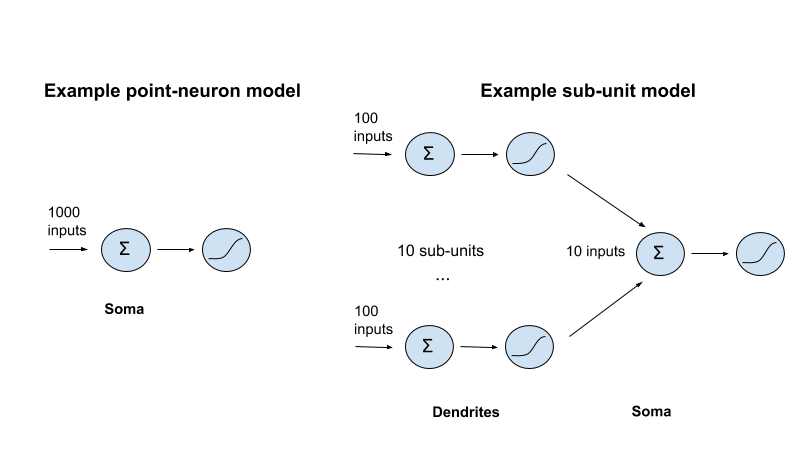
If we budget 1 FLOP per addition operation, and 10 per non-linearity (this is substantial overkill for certain non-linearities, like a ReLU),[220]From Open Philanthropy’s non-verbatim notes from a conversation with Dr. Paul Christiano: “A ReLU costs less than a FLOP. Indeed, it can be performed with many fewer transistors than a multiply of equivalent precision” (p. 6). See here for some discussion of the FLOPs costs of a tanh, … Continue reading we get the following budgets:
Point neuron model:
Soma: 1000 FLOPs (additions) + 10 FLOPs (non-linearity)
Total: 1010 FLOPs
Sub-unit model:
Dendrites: 10 (subunits) × (100 FLOPs (additions) + 10 FLOPs (non-linearity))
Soma: 10 FLOPs (additions) + 10 FLOPs (non-linearity)
Total: 1120 FLOPs
The totals aren’t that different (in general, the sub-unit model requires 11 additional FLOPs per sub-unit), even if the sub-unit model can do more interesting things. And if the tree-structure caps the number of non-linearities (and hence, sub-units) at the number of inputs, then the maximum increase is a factor of ~11×.[221] This factor is centrally determined by the ratio of FLOPs per input to FLOPs per non-linearity. This is 10x in the example above, but this is on the high end for non-linearities in ANNs. This story would alter if, for example, subunits could be fully connected, with each receiving all synaptic inputs, or all the outputs from subunits in a previous layer. But this fits poorly with a tree structured physiology.
Note, though, that the main upshot of this argument is that dendritic non-linearities won’t add that much computation relative to a model that budgets 1 FLOP per input connection per time-step. Our budget for synaptic transmission above, however, was based on spikes through synapses per second, not time-steps per synapse per second. In that context, if we assume that dendritic non-linearities need to be computed every time-step, then adding e.g. 100 or 1000 extra dendritic non-linearities per neuron could easily increase our FLOP/s budget by 100 or 1000x (see endnote for an example).[222]Thus, for example, assuming 1000 inputs and a 1 Hz average firing rate, on average there will be one spike through synapse per 1 ms timestep. If we budget 1 FLOP per spike through synapse, but assume 100 dendritic sub-units, each performing non-linearities on 10 synaptic input connections each, and … Continue reading That said, my impression is that many actual ANN models of dendritic computation use fewer sub-units, and it may be possible to avoid computing firing decisions/dendritic non-linearities every time-step as well – see brief discussion in section 2.1.2.5.
Cortical neurons as deep neural networks
What about evidence for larger FLOP/s costs from dendritic computation? One interesting example is Beniaguev et al. (2020), who found that they needed a very large deep neural network (7 layers, 128 channels per layer) to accurately predict the outputs of a detailed biophysical model of a cortical neuron, once they added conductances from a particular type of receptor (NMDA receptors).[223]Beniaguev et al. (2020): “A thorough search of configurations of deep and wide fully-connected neural network architectures (FCNs) have failed to provide a good fit to the I/O characteristics of the L5PC model. These failures suggest a substantial increase in the complexity of I/O transformation … Continue reading Without these conductances, they could do it with a much smaller network (a fully connected DNN with 128 hidden units and only one hidden layer), suggesting that it’s the dynamics introduced by NMDA-conductances in particular, as opposed to the behavior of the detailed biophysical model more broadly, that make the task hard.[224]Beniaguev et al. (2020): “We hypothesized that removing NMDA dependent synaptic currents from our L5PC model will significantly decrease the size of the respective DNN… after removing the NMDA voltage dependent conductance, such that the excitatory input relies only on AMPA mediated … Continue reading
This 7-layer network requires a lot of FLOPs: roughly 2e10 FLOP/s per cell.[225]Here’s my estimate, which the lead author tells me looks about right. 1st layer: 1278 synaptic inputs × 35 × 128 = 5.7 million MACCs (from line 140 and lines 179-180 here); Next 6 layers: 6 layers × 128 × 35 × 128 = 3.4 million MACCs. Total per ms: ~ 10 million MACCs. Total per second: ~10 … Continue reading Scaled up by 1e11 neurons, this would be ~2e21 FLOP/s overall. And these numbers could yet be too small: perhaps you need greater temporal/spatial resolution, greater prediction accuracy, a more complex biophysical model, etc., not to mention learning and other signaling mechanisms, in order to capture what matters.
I think that this is an interesting example of positive evidence for very high FLOP/s estimates. But I don’t treat it as strong evidence on its own. This is partly out of general caution about updating on single studies (or even a few studies) I haven’t examined in depth, especially in a field as uncertain as neuroscience. But there are also a few more specific ways these numbers could be too high:
- It may be possible to use a smaller network, given a more thorough search. Indeed, the authors suggest that this is likely, and have made data available to facilitate further efforts.[226]Beniaguev et al. (2020) (p. 15):It is important to emphasize that, due to optimization, the complexity measure described above is an upper bound of the true computational complexity of the I/O of a single neuron, i.e., it is possible that there exists a much smaller neural network that could mimic … Continue reading
- They focus on predicting both membrane potential and individual spikes very precisely.
- This is new (and thus far unpublished) work, and I’m not aware of other results of this kind.
The authors also suggest an interestingly concrete way to validate their hypothesis: namely, teach a cortical L5 pyramidal neuron to implement a function that this kind of 7-layer network can implement, such as classifying handwritten digits.[227]Beniaguev et al. (2020): “now that we estimate that a cortical L5 pyramidal neuron is equivalent to a deep network with 7 hidden layers, this DNN could be used to teach the respective neuron to implement a function which is in the scope of the capabilities of such a network, such as classifying … Continue reading If biological neurons can perform useful computational tasks thought to require very large neural networks to perform, this would indeed be very strong evidence for capacities exceeding what simple models countenance.[228] Though see Open Philanthropy’s non-verbatim notes from a conversation with Dr. Paul Christiano: “Dr. Christiano is very skeptical of the hypothesis that a single, biological cortical neuron could be used to classify handwritten digits” (p. 6). That said, “X is needed to predict the behavior of Y” does not imply that “Y can do anything X can do” (consider, for example, a supercomputer and a hurricane).
Overall, I think that dendritic computation is probably the largest source of uncertainty about the FLOP/s costs of firing decisions. I find the Beniaguev et al. (2020) results suggestive of possible lurking complexity; but I’m also moved somewhat by the relative simplicity of some common abstract models of dendritic computation, by the tree-structure argument above, and by experts who thought dendrites unlikely to imply a substantial increase in FLOP/s.
Crabs, locusts, and other considerations
Here are some other considerations relevant to the FLOP/s costs of firing decisions.
Other experimentally accessible circuits
The retina is not the only circuit where we have (a) some sense of what task it’s performing, and (b) relatively good experimental access. Here are two others I looked at that seem amenable to simplified modeling.
- A collection of ~30 neurons in the decapod crustacean stomach create rhythmic firing patterns that control muscle movements. Plausibly, maintaining these rhythms is the circuit’s high-level task.[229]From Open Philanthropy’s non-verbatim notes from a conversation with Prof. Eve Marder: “You can see maintaining these rhythms as the high-level function that the circuit is performing at a given time (transitions between modes of operation are discussed below). Neuroscientists had a wiring … Continue reading Such rhythms can be modeled well using single-compartment, Hodgkin-Huxley-type neuron models.[230]From Open Philanthropy’s non-verbatim notes from a conversation with Prof. Eve Marder: “Prof. Marder and her collaborators have used single-compartment conductance models to replicate the rhythms in the stomatogastric ganglion” (p. 4). And from Open Philanthropy’s non-verbatim notes from … Continue reading And naively, it seems to me like they could be re-implemented directly without using neuron models at all.[231]E.g., if what matters about these rhythms is that just that units activate in a certain regular, rhythmic sequence (I’m not sure about the details here, and the full range of dynamics that matter could be much more complicated), it seems possible to create this sort of sequence in a very … Continue reading What’s more, very different biophysical parameters (for example, synapse strengths and intrinsic neuron properties) result in very similar overall network behavior, suggesting that replicating task-performance does not require replicating a single set of such parameters precisely.[232]Prinz et al. (2004): “To determine how tightly neuronal properties and synaptic strengths need to be tuned to produce a given network output, we simulated more than 20 million versions of a three-cell model of the pyloric network of the crustacean stomatogastric ganglion using different … Continue reading That said, Prof. Eve Marder, an expert on this circuit, noted that the circuit’s biophysical mechanisms function in part to ensure smooth transitions between modes of operation – transitions that most computational models cannot capture.[233]From Open Philanthropy’s non-verbatim notes from a conversation with Prof. Eve Marder: “Biology has found a series of mechanisms that allow the system to transition smoothly between different modes of operation. For example, you can walk slowly or quickly. Although eventually you will change … Continue reading
- In a circuit involved in locust collision avoidance, low-level biophysical dynamics in the dendrites and cell body of a task-relevant neuron are thought to implement high-level mathematical operations (logarithm, multiplication, addition) that a computational model could replicate directly.[234]Locusts jump out of the way when you show them a “looming stimulus” – that is, a visual stimulus that grows in size in a manner that mimics an object on a collision course with the locust (see videos here and slower-motion here). In a particular locust neuron known as the lobula giant … Continue reading
I expect that further examination of the literature would reveal other examples in this vein.[235]See Fig 1 in Jadi et al. (2014) for some other examples of circuit models using point neuron models. They cite Raymond et al. (1996) for cerebellar circuit models; Raphael et al. (2010) for a model of the spinal cord; and Crick (1984) for a model of attention. Grid cells might be another … Continue reading
Selection effects
Neuroscientific success stories might be subject to selection effects.[236]From Open Philanthropy’s non-verbatim notes from a conversation with Dr. Stephen Larson: “There may be selection bias at work in appeals to the success of simple models in some contexts as evidence for their adequacy in general. With respect to phenomena that simple models have thus far failed … Continue reading For example, the inference “A, B, and C can be captured with simple models, therefore probably X, Y, and Z can too” is bad if the reason X, Y, and Z haven’t yet been so captured is that they can’t be.
However, other explanations may also be available. For example, it seems plausible to me we’ve had more success in peripheral sensory/motor systems than deeper in the cortex because of differences in the ease with which task-relevant inputs and outputs can be identified, measured, and manipulated, rather than differences in the computation required to run adequate models of neurons in those areas.[237]I’m partly influenced here by discussions with Dr. Adam Marblestone, see Open Philanthropy’s non-verbatim notes from a conversation with Dr. Adam Marblestone: “Dr. Marblestone does not think that selection effects nullify the evidence provided by our understanding of peripheral sensory and … Continue reading And FLOP/s requirements do not seem to be the major barrier to e.g. C. elegans simulation.[238]From Open Philanthropy’s non-verbatim notes from a conversation with Dr. Stephen Larson, who works on the OpenWorm project: “Despite its small size, we do not yet have a model that captures even 50% of the biological behavior of the C. elegans nervous system. This is partly because we’re … Continue reading
Evolutionary history
Two experts (one physicist, one neuroscientist) mentioned the evolutionary history of neurons as a reason to think that they don’t implement extremely complex computations. The basic thought here seemed to be something like: (a) neurons early in evolutionary history seem likely to have been doing something very simple (e.g., basic stimulus-response behavior), (b) we should expect evolution to tweak and recombine these relatively simple components, rather than to add a lot of complex computation internal to the cells, and (c) indeed, neurons in the human brain don’t seem that different from neurons in very simple organisms.[239]From Open Philanthropy’s non-verbatim notes from a conversation with Dr. Adam Marblestone: “Some neural circuits, like ones in the spinal cord, are very simple. And one can imagine primitive synapses, involved in primitive computations like “if you get some dopamine, move this part of the … Continue reading I haven’t looked into this, but it seems like an interesting angle.[240]Though see also comments from Open Philanthropy’s non-verbatim notes from a conversation with Prof. Erik De Schutter: “The brain was not engineered. Rather, it evolved, and evolution works by adding complexity, rather than by simplification. There are good reasons for this complexity. In order … Continue reading
Communication bottlenecks
A number of experts mentioned limitations on the bits that a neuron receives as input and sends as output (limitations imposed by e.g. firing precision, the number of distinguishable synaptic states, etc.) as suggestive of a relatively simple input-output mapping.[241]Dr. Dario Amodei suggests considerations in this vein, though I’m not sure I’ve understood what he has in mind. See also Open Philanthropy’s non-verbatim notes from a conversation with Prof. Jared Kaplan: “most of his probability mass on the hypothesis that most of the computation … Continue reading
I’m not sure exactly how this argument works (though I discuss one possibility in the communication method section). In theory, very large amounts of computation can be required to map a relatively small number of possible inputs (e.g., the product of two primes, a boolean formula) to a small a number of possible outputs (e.g., the prime factors, a bit indicating whether the formula is satisfiable).[242]From Open Philanthropy’s non-verbatim notes from a conversation with Dr. Paul Christiano: “Neurons receive only a limited number of bits in, and they output only a limited number of bits. However, in principle, you can imagine computational elements receiving encodings of computationally … Continue reading For example, RSA-240 is ~800 bits (if we assume 1000-10,000 input synapses, each receiving 1 spike/s in 1 of 1000 bins, a neuron would be receiving ~10-100k bits/s),[243]Here I’m using a rough estimation method suggested by Dr. Paul Christiano, from Open Philanthropy’s non-verbatim notes from a conversation with Dr. Paul Christiano: “You can roughly estimate the bandwidth of axon communication by dividing the firing rate by the temporal resolution of … Continue reading but it took ~900 core years on a 2.1 Ghz CPU to factor.[244] See here, and more discussion of the difficulties here. And the bits that the human brain as a whole receives and outputs may also be quite limited relative to the complexity of its information-processing (Prof. Markus Meister suggested ~10-40 bits per second for various motor outputs).[245]From Open Philanthropy’s non-verbatim notes from a conversation with Prof. Markus Meister: “Prof. Meister thinks that people often overestimate the sophistication of the tasks that humans perform, which tend to involve low-bandwidth outputs. People have measured the bits per second involved in … Continue reading
Of course, naively, neurons (indeed, brains) don’t seem to be factorizing integers. Indeed, in general, I think this may well be a good argument, and I welcome attempts to make it more explicit and quantified. Suppose, for example, that a neuron receives ~10-100k bits/s and outputs ~10 bits/s. What would this suggest about the FLOP/s required to reproduce the mapping, and why?
Ability to replicate known types of neuron behavior
According to Izhikevich (2004), some neuron models, such as simple integrate-and-fire models, can’t replicate known types of neuron behaviors, some of which (like adaptations in spike frequency over time, and spike delays that depend on the strength of the inputs)[246]Izhikevich (2004): “The most common type of excitatory neuron in mammalian neocortex, namely the regular spiking (RS) cell, fires tonic spikes with decreasing frequency, as in Fig. 1(f). That is, the frequency is relatively high at the onset of stimulation, and then it adapts. Low-threshold … Continue reading seem to me plausibly important to task-performance:[247]Izhikevich (2004): “The most efficient is the I&F model. However, the model cannot exhibit even the most fundamental properties of cortical spiking neurons, and for this reason it should be avoided by all means. The only advantage of the I&F model is that it is linear, and hence amenable … Continue reading

Note, though, that Izhikevich suggests that his own model can capture these behaviors, for 13 FLOPs per ms.
Simplifying the Hodgkin-Huxley model
Some experts argue that the Hodgkin-Huxley model can be simplified:
- Prof. Dong Song noted that the functional impacts of its ion channel dynamics are highly redundant, suggesting that you can replicate the same behavior with fewer equations.[248]From Open Philanthropy’s non-verbatim notes from a conversation with Prof. Dong Song: “The functional impact of ion channel dynamics in the context of a Hodgkin-Huxley model is highly redundant. This makes Prof. Song think that Hodgkin-Huxley models can be simplified – e.g. you can replicate … Continue reading
- Izhikevich (2003) claims that “[His simplified neuron model] consists of only two equations and has only one nonlinear term, i.e., v2. Yet … the difference between it and a whole class of biophysically detailed and accurate Hodgkin–Huxley-type models, including those consisting of enormous number of equations and taking into account all possible information about ionic currents, is just a matter of coordinate change.”[249]He cites Hoppensteadt and Izhikevich (2001), in which he goes into more detail: “Briefly, a model is canonical for a family if there is a continuous change of variables that transforms any other model from the family into this one, as we illustrate in Figure 1. For example, the entire family of … Continue reading
ANNs and interchangeable non-linearities
Artificial neural networks (ANNs) have led to breakthroughs in AI, and we know they can perform very complex tasks.[250]Here is a summary of recent AI progress from Hassabis et al. (2017): “In AI, the pace of recent research has been remarkable. Artificial systems now match human performance in challenging object recognition tasks (Krizhevsky et al. (2012)) and outperform expert humans in dynamic, adversarial … Continue reading Yet the individual neuron-like units are very simple: they sum weighted inputs, and their “firing decisions” are simple non-linear operations, like a ReLU.[251] See Kriegeskorte (2015) and Nielsen’s “Neural Networks and Deep Learning” for general introductions.
The success of ANNs is quite compatible with the biological neurons doing something very different. And comparisons between brains and exciting computational paradigms can be over-eager.[252]From Open Philanthropy’s non-verbatim notes from a conversation with Prof. Eric Jonas: “Prof. Jonas does not think that there is a clear meaning to the claim that the brain is a deep learning system, and he is unconvinced by the argument that ‘the brain is doing optimization, and what is … Continue reading Still, knowing that ANN-like units are useful computational building-blocks makes salient the possibility that biological neurons are useful for similar reasons. Alternative models, including ones that incorporate biophysical complications that ANNs ignore, cannot boast similar practical success.
What’s more, the non-linear operations used in artificial neurons are, at least to some extent, interchangeable.[253]From Open Philanthropy’s non-verbatim notes from a conversation with Prof. Anthony Zador: “In the early days of neural networks, people thought you needed sigmoid activation functions, and that piecewise linear models could not work because they are not differentiable. But it turns out that … Continue reading That is, instead of a ReLU, you can use e.g., a sigmoid (though different operations have different pros and cons). If we pursue the analogy with firing decisions, this interchangeability might suggest that the detailed dynamics that give rise to spiking are less important than the basic function of passing synaptic inputs through some non-linearity or other.
On a recent podcast, Dr. Matthew Botvinick also mentions a chain of results going back to the 1980s showing that the activity in the units of task-trained deep learning systems bears strong resemblance to the activity of neurons deep in the brain. I discuss a few recent visual cortex results in this vein in Section 3.2, and note a few other recent results in Section 3.3.[254]See Matthew Botvinick’s comments in this podcast: “I consider the networks we use in deep learning research to be a reasonable approximation to the mechanisms that carry information in the brain…If you go back to the 1980s, there’s an unbroken chain of research in which a particular … Continue reading Insofar as a much broader set of results in this vein is available, that seems like relevant evidence as well.
Intuitive usefulness
One of our technical advisors, Dr. Paul Christiano, noted that from a computer science perspective, the Hodgkin-Huxley model just doesn’t look very useful. That is, it’s difficult to describe any function for which (a) this model is a useful computational building block, and (b) its usefulness arises from some property it has that simpler computational building blocks don’t.[255] From Open Philanthropy’s non-verbatim notes from a conversation with Dr. Paul Christiano, (p. 6). Perhaps something similar could be said of even more detailed biophysical models.
Note, though, advocates of large compute burdens need not argue that actual biophysical models themselves are strictly necessary; rather, they need only argue for the overall complexity of a neuron’s input-output transformation.
Noise bounds
Various experts suggest that noise in the brain may provide an upper bound on the compute required to do what it does.[256]Sandberg (2013): “The noise level in the nervous system is fairly high, with spike-timing variability reaching milliseconds due to ion channel noise. Perceptual thresholds and motor precision are noise limited. Various noise management solutions such as redundant codes, averaging and bias have … Continue reading However, I’m not sure how to identify this bound, and haven’t tried.
Expert opinion and practice
There is no consensus in neuroscience about what models suffice to capture task-relevant neuron behavior.[257]Gerstner and Naud (2009): “Opinions strongly diverge on what constitutes a good model of a neuron” (p. 379). Herz et al. (2006): “Even today, it remains unclear which level of single-cell modeling is appropriate to understand the dynamics and computations carried out by such large systems … Continue reading
A number of experts indicated that in practice, the field’s emphasis is currently on comparatively simple models, rather than on detailed modeling.[258]From Open Philanthropy’s non-verbatim notes from a conversation with Prof. Erik De Schutter: “Modeling neural networks at the level of simple spiking neuron models or rate-based models is very popular. Prof. De Schutter thinks the field would benefit from a greater diversity of approaches” … Continue reading But this evidence is indirect. After all, the central question a neuroscientist needs to ask is not (a) “what model is sufficient, in principle, to replicate task-relevant behavior?”, but rather (b) “what model will best serve the type of neuroscientific understanding I am aiming to advance, given my constraints?”.
Indeed, much discussion of model complexity is practical: it is often said that biophysical models are difficult to compute, fit to data, and understand; that simpler models, while better on these fronts, come at the cost of biological realism; and that the model you need depends on the problem at hand.[259]Herz et al. (2006): “The appropriate level of description depends on the particular goal of the model. Indeed, finding the best abstraction level is often the key to success” (p. 80). Pozzorini et al. (2015): “Detailed biophysical models with stochastic ion channel dynamics can in principle … Continue reading Thus, answers to (a) and (b) can come apart: you can think that ultimately, we’ll need complex models, but that simpler ones are more useful given present constraints; or to that ultimately, simplifications are possible, but detailed modeling is required to identify them.[260]From Open Philanthropy’s non-verbatim notes from a conversation with Prof. Erik De Schutter: “The best way forward is to try to explore and understand the function of the brain’s underlying mechanisms – a project that may eventually lead to an understanding of what can be simplified. But … Continue reading
Still, some experts answer (a) explicitly. In particular:
- A number of experts I spoke to expected comparatively simple models (e.g., simpler than Hodgkin-Huxley) to be adequate.[261]From Open Philanthropy’s non-verbatim notes from a conversation with Prof. Anthony Zador (p. 1-2):Prof. Zador believes that integrate-and-fire neuron models, or something like them, are adequate to capture the contribution of a neuron to the brain’s information-processing. He does not think … Continue readingI expect many computational neuroscientists who have formed opinions on the topic (as opposed to remaining agnostic) to share this view.[262]A number of experts we engaged with indicated that many in the field are sympathetic to the adequacy of models less compute-intensive than single-compartment Hodgkin-Huxley (though we have very few comments in this respect publicly documented), and it fits with my impressions more broadly. See … Continue reading
- Various experts suggest that some more detailed biophysical models are adequate.[263]Jonathan Pillow says in a lecture: “Obviously if I simulate the entire brain using multi-compartment Hodkin-Huxley models that describe the opening and closing of every channel, clearly that model has the capacity to do anything that the brain can do” (16:10). Pozzorini et al. (2015) write: … Continue reading
- In an informal poll of participants at a 2007 workshop on Whole Brain Emulation, the consensus appeared to be that a level of detail somewhere between a “spiking neural network” and the “metabolome” would be adequate (strong selection effects likely influenced who was present).[264]Workshop participants included: John Fiala, Robin Hanson, Kenneth Jeffrey Hayworth, Todd Huffman, Eugene Leitl, Bruce McCormick, Ralph Merkle, Toby Ord, Peter Passaro, Nick Shackel, Randall A. Koene, Robert A. Freitas Jr and Rebecca Roache. From a brief google, a number of these people appear to be … Continue reading
A number of other experts I spoke with expressed more uncertainty, agnosticism, and sympathy towards higher end estimates.[265]From Open Philanthropy’s non-verbatim notes from a conversation with Dr. Stephen Larson (p. 5): On the basis of his experience at OpenWorm thus far, Dr. Larson thinks it unlikely that very simplified neuron models (e.g., integrate-and-fire neurons, or models akin to the artificial neurons used … Continue reading And many (regardless of specific opinion) suggested that views about this topic (including, sometimes, their own) can emerge in part from gut feeling, a desire for one’s own research to be important/tractable, and/or from the tradition and assumptions one was trained in.[266]From Open Philanthropy’s non-verbatim notes from a conversation with Prof. Erik De Schutter: Many common simplifications do not have solid scientific foundations, and are more at the level of ‘the way we do things.’ From Open Philanthropy’s non-verbatim notes from a conversation with … Continue reading
Overall FLOP/s for firing decisions
Where does this leave us in terms of overall FLOP/s for firing decisions? Here’s a chart with some examples of possible levels of complexity, scaled up to the brain as a whole:
| ANCHOR | FLOPS | SIZE OF TIMESTEP | FLOP/S FOR 1E11 NEURONS |
|---|---|---|---|
| ReLU | 1 FLOP per operationr[267]From Open Philanthropy’s non-verbatim notes from a conversation with Dr. Paul Christiano:”A ReLU costs less than a FLOP. Indeed, it can be performed with many fewer transistors than a multiply of equivalent precision” (p. 6) | 10 ms[268] This number is just a ballpark for lower temporal resolutions. For example, it’s the resolution used by Maheswaranathan et al. (2019) | 1e13 |
| Izhikevich spiking neuron model | 13 FLOPs per ms[269] Izhikevich (2004), (p. 1068) | 1 ms[270]Izhikevich (2004) seems to be assuming at least 1000 time-steps per second: “It takes only 13 floating point operations to simulate 1 ms of the model, so it is quite efficient in large-scale simulations of cortical networks. When and (a,b,c,d) = (0.2, 2, -56, -16) and I = -99, the model has … Continue reading | ~1e15 |
| Single compartment Hodgkin-Huxley model | 120 FLOPs per .1 ms[271] Izhikevich (2004), (p. 1069). | .1 ms[272]The FLOPs estimate for the Hodgkin-Huxley model given in Izhikevich (2004) appears to assume at least 10,000 timesteps/sec: “It takes 120 floating point operations to evaluate 0.1 ms of model time (assuming that each exponent takes only ten operations), hence, 1200 operations/1 ms” (p. 1069). … Continue reading | ~1e17 |
| Beniaguev et al. (2020) DNN | 1e7 FLOPs per ms[273]Here’s my estimate, which the lead author of the paper tells me looks about right. 1st layer: 1278 synaptic inputs × 35 × 128 = 5.7 million MACCs (from line 140 and lines 179-180 here); Next 6 layers: 6 layers × 128 × 35 × 128 = 3.4 million MACCs. Total per ms: ~ 10 million MACCs. Total per … Continue reading | 1 ms | ~1e21 |
| Hay et al. (2011) detailed L5PC model | 1e10 FLOPs per ms?[274]This is a very loose estimate, based on scaling up the estimate for the Beniaguev et al. (2020) DNN by ~1000x, on the basis of their reporting, in the 2019 version of the paper, that “In our tests we obtained a factor of ~2000 speed up when using the DNN instead of its compartmental-model … Continue reading | ? | 1e24? |
Even the lower-end numbers here are competitive with the budgets for synaptic transmission above (1e13-1e17 FLOP/s). This might seem surprising, given the difference in synapse and neuron count. But as I noted at the beginning of the section, the budgets for synaptic transmission were based on average firing rates; whereas I’m here assuming that firing decisions must be computed once per time-step (for some given size of time-step).[275]This is somewhat analogous to the approach taken by Ananthanarayanan et al. (2009): “The basic algorithm of our cortical simulator C2 [2] is that neurons are simulated in a clock-driven fashion whereas synapses are simulated in an event-driven fashion. For every neuron, at every simulation time … Continue reading
This assumption may be mistaken. Dr. Paul Christiano, for example, suggested that it would be possible to accumulate inputs over some set of time-steps, then calculate what the output spike pattern would have been over that period.[276]From Open Philanthropy’s non-verbatim notes from a conversation with Dr. Paul Christiano: “Dr. Christiano expects that in modeling a neuron’s input-output function, one would not need to compute, every time-step, whether or not the neuron fires during that time-step. Rather, you could … Continue reading And Sarpeshkar (2010) appears to assume that the FLOP/s he budgets for firing decisions (enough for 1 ms of Hodgkin-Huxley model) need only be used every time the neuron spikes.[277]Sarpeshkar (2010) employs what appears to be a single-compartment Hodgkin-Huxley model of firing decisions as a lower bound (he cites Izhikevich (2004), and uses an estimate of 1200 FLOPs per firing decision – the number that Izhikevich gives for running a Hodgkin-Huxley model for one ms (see … Continue reading If something like this is true, the numbers would be lower.
Other caveats:
- I’m leaning heavily on the FLOPs estimates in Izhikevich (2004), which I haven’t verified.
- Actual computation burdens for running e.g. a Hodgkin-Huxley model depend on implementation details like platform, programming language, integration method, etc.[278]From Open Philanthropy’s non-verbatim notes from a conversation with Prof. Eve Marder: “the computational power necessary to run e.g. a full Hodgkin-Huxley model depends a lot on implementation: e.g., what platform you use, what language you’re using, what method of integration, and what … Continue reading
- In at least some conditions, simulations of integrate-and-fire neurons can require very fine grained temporal resolution (e.g., 0.001 ms) to capture various properties of network behavior.[279]See Hansel et al. (1998): “It is shown that very small time steps are required to reproduce correctly the synchronization properties of large networks of integrate-and-fire neurons when the differential system describing their dynamics is integrated with the standard Euler or second-order … Continue reading Temporal resolutions like this would increase the numbers above considerably. However, various other simulations using simplified spiking neuron models, such as the leaky-integrate-and-fire simulations run by Prof. Chris Eliasmith (which actually perform tasks like recognizing numbers and predicting sequences of them), use lower resolutions.[280]From Open Philanthropy’s non-verbatim notes from a conversation with Prof. Chris Eliasmith: “Prof. Eliasmith typically uses 1 ms time-steps in the simulations he builds” (p. 3); and Eliasmith et al. (2012) use leaky-Integrate-and-fire models (see p. 16 of the supplementary … Continue reading
- The estimate above for Hay et al. (2011) is especially rough.[281]It’s based on scaling up the estimate for the Beniaguev et al. (2020) DNN by ~1000x, on the basis of their reporting, in the 2019 version of the paper, that “In our tests we obtained a factor of ~2000 speed up when using the DNN instead of its compartmental-model counterpart” (p. 15). In … Continue reading
- The high end of this chart is not an upper bound on modeling complexity. Biophysical modeling can in principle be arbitrarily detailed.
Overall, my best guess is that the computation required to run single-compartment Hodgkin-Huxley models of every neuron in the brain (1e17 FLOP/S, on the estimate above) is overkill for capturing the task-relevant dimensions of firing decisions. This is centrally because:
- Efforts to predict neuron behavior using simpler models (including simplified models of dendritic computation) appear to have had a decent amount of success (though these results also have many limitations, and I’m not in a great position to evaluate them).
- With the exception of Beniaguev et al. (2020), I don’t see much positive evidence that dendritic computation alters this picture dramatically.
- I find some of the considerations canvassed in Section 2.1.2.3 (other simple circuits; the success of ANNs with simple, interchangeable non-linearities) suggestive; and I think that others I don’t understand very well (e.g., communication bottlenecks, mathematical results showing that the Hodgkin-Huxley equations can be simplified) may well be quite persuasive on further investigation.
- My impression is that a substantial fraction (maybe a majority?) of computational neuroscientists who have formed positive opinions about the topic (as opposed to remaining agnostic) would also think that single-compartment Hodgkin-Huxley is overkill for capturing task-performance (though it may be helpful for other forms of neuroscientific understanding).
Thus, I’ll use 1e17 FLOP/s as a high-end estimate for firing decisions.
The Izhikevich spiking neuron model estimate (1e15 FLOP/s) seems to me like a decent default estimate, as it can capture more behaviors than a simple integrate-and-fire model, for roughly comparable FLOP/s (indeed, Izhikevich seems to argue that it can do anything a Hodgkin-Huxley model can). And if simpler operations (e.g., a ReLU) and/or lower time resolutions are adequate, we’d drop to something like 1e13 FLOP/s, possibly lower. I’ll use 1e13 FLOP/s as a low end, leaving us with an overall range similar to the range for synaptic transmission: 1e13 to 1e17 FLOP/s.
Learning
Thus far, we have been treating the synaptic weights and firing decision mappings as static over time. In reality, though, experience shapes neural signaling in a manner that improves task performance and stores task-relevant information. I’ll call these changes “learning.”
Some of these may proceed via standard neuron signaling (for example, perhaps firing patterns in networks with static weights could store short-term memories).[282]From Open Philanthropy’s non-verbatim notes from a conversation with Dr. Adam Marblestone: “It might be that all of the neurons and synapses in the brain are there in order to make the brain more likely to converge on a solution while learning, but that once learning has taken place, the brain … Continue reading But the budgets thus far already cover this. Here I’ll focus on processes that we haven’t yet covered, but which are thought to be involved in learning. These include:
- Synaptic weights change over time (“synaptic plasticity”). These changes are often divided into categories:
- Short-term plasticity (e.g., changes lasting from hundreds of milliseconds to a few seconds).
- Long-term plasticity (changes lasting longer).[283]Tsodyks and Wu (2013): “Compared with long-term plasticity (Bi and Poo (2001)), which is hypothesized as the neural substrate for experience-dependent modification of neural circuit, STP has a shorter time scale, typically on the order of hundreds to thousands of milliseconds.” See … Continue reading
- The type of synaptic plasticity neurons exhibit can itself change (“meta-plasticity”).
- The electric properties of the neurons (for example, ion channel expression, spike threshold, resting membrane potential) also change (“intrinsic plasticity”).[284]Cudmore and Desai (2008): “Intrinsic plasticity is the persistent modification of a neuron’s intrinsic electrical properties by neuronal or synaptic activity. It is mediated by changes in the expression level or biophysical properties of ion channels in the membrane, and can affect such diverse … Continue reading
- New neurons, synapses, and dendritic spines grow over time, and old ones die.[285] See e.g. Munno and Syed (2003), Ming and Song (2011), Grutzendler et al. (2002), Holtmaat et al. (2005).
Such changes can be influenced by many factors, including pre-synaptic and post-synaptic spiking,[286] See e.g. Markram et al. (1997). receptor activity in the post-synaptic dendrite,[287] See Luscher and Malenka (2012). the presence or absence of various neuromodulators,[288] See e.g. Gerstner et al. (2018), and Nadim and Bucher (2014). interactions with glial cells,[289] See Monday et al. (2018) (p. 7-8). chemical signals from the post-synaptic neuron to the pre-synaptic neuron,[290] See Tao and Poo (2001). and gene expression.[291] See Yap and Greenberg (2018). There is a lot of intricate molecular machinery plausibly involved,[292] See Bhalla (2014), Figure 1, for a diagram depicting some of this machinery. which we don’t understand well and which can be hard to access experimentally[293]From Open Philanthropy’s non-verbatim notes from a conversation with Prof. Blake Richards: “Some neuroscientists are interested in the possibility that a lot of computation is occurring via molecular processes in the brain. For example, very complex interactions could be occurring in a … Continue reading (though some recent learning models attempt to incorporate it).[294]Lahiri and Ganguli (2013): Lahiri and Ganguli (2013): “To understand the functional contribution of such molecular complexity to learning and memory, it is essential to expand our theoretical conception of a synapse from a single scalar to an entire dynamical system with many internal molecular … Continue reading And other changes in the brain could be relevant as well.[295] Activity-dependent myelination might be one example (see e.g. Faria et al. (2019)).
Of course, many tasks (say, tying your shoes) don’t require much learning, once you know how to do them. And many tasks are over before some of the mechanisms above have had time to have effects, suggesting that such mechanisms can be left out of FLOP/s budgets for those tasks.[296]Though short-term plasticity is both (a) fairly fast and (b) possibly involved in working memory, which many tasks require. See also Sandberg and Bostrom (2008): “Since neurogenesis occurs on fairly slow timescales (> 1 week) compared to brain activity and normal plasticity, it could probably … Continue reading
But learning to perform new tasks, sometimes over long timescales, is itself a task that the brain can perform. So a FLOP/s estimate for any task that the brain can perform needs to budget FLOP/s for all forms of learning.
How many FLOP/s? Here are a few considerations.
Timescales
Some of the changes involved in learning occur less frequently than spike through synapses. Growing new neurons, synapses, and dendritic spines is an extreme example. At a glance, the number of new neurons per day in adult humans appears to be on the order of hundreds or less;[297]Sorrells et al. (2018): “In humans, some studies have suggested that hundreds of new neurons are added to the adult dentate gyrus every day, whereas other studies find many fewer putative new neurons.” See also Moreno-Jimenez et al. (2019): “we identified thousands of immature neurons in the … Continue reading and Zuo et al. (2005) report that over two weeks, only 3%-5% of dendritic spines in adult mice were eliminated and formed (though Prof. Erik De Schutter noted that networks of neurons can rewire themselves over tens of minutes).[298]Zuo et al. (2005): “In adult mice (4-6 months old), 3%-5% of spines were eliminated and formed over 2 weeks in various cortical regions. Over 18 months, only 26% of spines were eliminated and 19% formed in adult barrel cortex” (from the abstract). From Open Philanthropy’s non-verbatim notes … Continue reading Because these events are so comparatively rare, I expect modeling their role in task-performance to be quite cheap relative to e.g. 1e14 spikes through synapses/sec.[299] Dr. Dario Amodei suggested considerations in this vein. This holds even if the number of FLOPs required per event is very large, which I don’t see strong reason to expect.
Something similar may apply to some other types of changes to e.g. synaptic weights and intrinsic neuron properties:
- Some long-term changes require building new biochemical machinery (receptors, ion channels, etc.), which seems resource-intensive relative to e.g. synaptic transmission (though I don’t have numbers here).[300] See e.g. this diagram of a potentiated synapse, illustrating an increased number of post-synaptic receptors This suggests limitations on frequency.
- If a given type of change lasts a long time in vivo (and hence, is not “reset” very frequently) or is triggered primarily by relatively rare events (e.g., sustained periods of high-frequency pre-synaptic spiking), this could also suggest such limitations.[301] Thus, for example, Bliss and Lømo (1973), in an early result related to long-lasting synaptic potentiation, use conditioning spike trains of 10-15 secs, and 3-4 seconds (p. 331).
- It seems plausible that some amount of stability is required for long-term information storage.[302] See discussion of the “stability – plasticity dilemma,” e.g. Mermillod et al. (2013). One possible solution is to use multiple dynamical variables operating on different timescales – see Benna and Fusi (2016).
More generally, some biochemical mechanisms involved in learning are relatively slow-moving. The signaling cascades triggered by some neuromodulators, for example, are limited by the speed of chemical diffusion, which Koch (1999) suggests extends their timescales to seconds or longer;[303]Koch (1999): “An important distinction between ionotropic and metabotropic receptors is their time scale. While members of the former class act rapidly, terminating within a very small fraction of a second, the speed of the latter class is limited by diffusion. Biochemical reactions can happen … Continue reading Bhalla (2014) characterizes various types of chemical computation within synapses as occurring on timescales of seconds;[304] See p. 32. Bhalla (2014) also suggests that chemical computation involves 1e6 “computations per second” per neuron. and Yap and Greenberg (2018) characterize gene transcription taking place over minutes as “rapid.”[305]Yap and Greenberg (2018): “Discovered by Greenberg and Ziff in 1984 (Greenberg and Ziff (1984)), the rapid and transient induction of Fos transcription provided the first evidence that mammalian cells could respond to the outside world within minutes by means of rapid gene transcription, in … Continue reading This too might suggest limits on required FLOP/s.
I discuss arguments that appeal to timescales in more detail in Section 2.3. As I note there, I don’t think these arguments are conceptually airtight, but I find them suggestive nonetheless, and I expect them to apply to many processes involved in learning.
That said, the frequency with which a given change occurs does not necessarily limit the frequency with which biophysical variables involved in the process need to be updated, or decisions made about what changes to implement as a result.[306]Indeed, certain models of synaptic plasticity explicitly include variables whose state is not immediately expressed in changes to synaptic efficacy (that is, in the size of the effect that a spike through that synapse has on a downstream neuron). See e.g. three-factor learning rules discussed … Continue reading What’s more, some forms of synaptic plasticity occur on short timescales, reflecting rapid changes in e.g. calcium or neurotransmitter in a synapse;[307]Tsodyks and Wu (2013): “Compared with long-term plasticity (Bi and Poo (2001)), which is hypothesized as the neural substrate for experience-dependent modification of neural circuit, STP has a shorter time scale, typically on the order of hundreds to thousands of milliseconds.” Cheng et al. … Continue reading and Bhalla (2014) notes that spike-timing dependent plasticity “requires sharp temporal discrimination of the order of a few milliseconds” (p. 32).
There is no consensus model for how the brain learns,[308]From Open Philanthropy’s non-verbatim notes from a conversation with Prof. Blake Richards: “it is very difficult to say at this point exactly how much compute would be required to model learning in the brain, because there is a lot of disagreement in the field as to how sophisticated the … Continue reading and the training required to create state of the art AI systems seems in various ways comparatively inefficient.[309]See Yann LeCun’s 2017 talk: “How does the brain learn so much so quickly?”, and Stuart Russell’s comments here: “I think another area where deep learning is clearly not capturing the human capacity for learning, is just in the efficiency of learning. I remember in the mid ’80s going … Continue reading There is debate over comparisons with learning algorithms like backpropagation[310]See e.g., Guerguiev et al. (2017), Bartunov et al. (2018), and Hinton (2011). From Guerguiev et al. (2017): “Backpropagation assigns credit by explicitly using current downstream synaptic connections to calculate synaptic weight updates in earlier layers, commonly termed ‘hidden layers’ … Continue reading (along with meta-debate about whether this debate is meaningful or worthwhile).[311]See e.g. David Pfau via twitter: “In 100 years, we’ll look back on theories of ‘how the brain does backpropagation’ the way we look at the luminiferous aether now.” See also Open Philanthropy’s non-verbatim notes from a conversation with Prof. Eric Jonas: “Prof. Jonas does not think … Continue reading
Still, different models can at least serve as examples of possible FLOP/s costs. Here are a few that came up in my research.
| LEARNING MODEL | DESCRIPTION | FLOP/S COSTS | EXPERT OPINION |
|---|---|---|---|
| Hebbian rules | Classic set of models. A synapse strengthens or weakens as a function of pre-synaptic spiking and post-synaptic spiking, possibly together with some sort of external modulation/reward.[312]See e.g. Gerstner et al. (2018) for some descriptions. From Open Philanthropy’s non-verbatim notes from a conversation with Dr. Adam Marblestone: “A lot of the learning models discussed in neuroscience are also significantly simpler than backpropagation: e.g., three-factor rules like “if … Continue reading | 3-5 FLOPs per synaptic update?[313]From Open Philanthropy’s non-verbatim notes from a conversation with Prof. Chris Eliasmith: “In the large scale brain simulations that Chris Eliasmith builds, he often uses an error-driven Hebbian rule, which computes updates to synaptic weights based on pre-synaptic activity, post-synaptic … Continue reading | Prof. Anthony Zador expected the general outlines to be correct.[314]From Open Philanthropy’s non-verbatim notes from a conversation with Prof. Anthony Zador: “We know the general outlines of the rules governing synaptic plasticity. The synapse gets stronger and weaker as a function of pre and post synaptic activity, and external modulation. There is a lot of … Continue reading Prof. Chris Eliasmith uses a variant in his models.[315]From Open Philanthropy’s non-verbatim notes from a conversation with Prof. Chris Eliasmith: “In the large scale brain simulations that Chris Eliasmith builds, he often uses an error-driven Hebbian rule, which computes updates to synaptic weights based on pre-synaptic activity, post-synaptic … Continue reading |
| Benna and Fusi (2016) | Models synapses as a dynamical system of variables interacting on multiple timescales. May help resolve the “stability-plasticity dilemma,” on which overly plastic synapses are too easily overwritten, but overly rigid synapses are unable to learn. May also help with online learning. | ~2-30x the FLOPs to run a model with one parameter per synapse? (very uncertain)[316]Kaplanis et al. (2018) add 30 extra dynamical variables per synapse, but manage to increase runtime by only 1.5-2 times relative to a control model, though I’m not sure about the details here. They note that “the complexity of the algorithm is O(mN), where N is the number of trainable … Continue reading | Some experts argue that shifting to synaptic models of this kind, involving dynamical interactions, is both theoretically necessary and biologically plausible.[317]See e.g. Lahiri and Ganguli (2013): “To understand the functional contribution of such molecular complexity to learning and memory, it is essential to expand our theoretical conception of a synapse from a single scalar to an entire dynamical system with many internal molecular functional … Continue reading |
| First order gradient descent methods | Use slope of the loss function to minimize the loss.[318] From Open Philanthropy’s non-verbatim notes from a conversation with Prof. Blake Richards: “First-order gradient descent methods, like back-propagation, use the slope of the loss function to minimize the loss” (p. 1-2). Widespread use in machine learning. Contentious debate about biological plausibility. | ~2× a static network. The learning step is basically a backwards pass through the network, and going forward and backward come at roughly the same cost.[319]From Open Philanthropy’s non-verbatim notes from a conversation with Prof. Blake Richards: “[For first-order gradient descent methods], learning is basically a backwards pass through the network, so the compute required scales linearly with the number of neurons and synapses in the network, … Continue reading | Prof. Konrad Kording, Prof. Barak Pearlmutter, and Prof. Blake Richards favored estimates based on this anchor/in this range of FLOP/s costs.[320]From Open Philanthropy’s non-verbatim notes from a conversation with Prof. Barak Pearlmutter: “Prof. Pearlmutter’s best-guess estimate was that the learning overhead (that is, the compute increase from moving from a non-adaptive system to an adaptive system) would be a factor of two. It … Continue reading |
| Second order gradient descent methods | Take into account not just the slope of the loss function, but also the curvature. Arguably better than gradient descent methods, but require more compute, so used more rarely.[321]From Open Philanthropy’s non-verbatim notes from a conversation with Prof. Blake Richards: “More sophisticated learning algorithms, such as second-order gradient methods, take into account not just the slope of the loss function gradient but also its curvature. These require more compute (the … Continue reading | Large. Compute per learning step scales as a polynomial with the number of neurons and synapses in a network.[322] See previous endnote. | Dr. Paul Christiano thought it very implausible that the brain implements a rule of this kind.[323] From Open Philanthropy’s non-verbatim notes from a conversation with Dr. Paul Christiano: “Based on his understanding of the brain’s physiology, Dr. Christiano thinks it extremely implausible that the brain could be implementing second-order optimization methods” (p. 7). Dr. Adam Marblestone had not seen any proposals in this vein.[324] From Open Philanthropy’s non-verbatim notes from a conversation with Dr. Adam Marblestone: “He has not seen proposals for how second-order gradient methods of learning could be implemented in the brain.” (p. 6). |
| Node-perturbation algorithms | Involves keeping/consolidating random changes to the network that result in reward, and getting rid of changes that result in punishment. As the size of a network grows, these take longer to converge than first-order gradient methods.[325]From Open Philanthropy’s non-verbatim notes from a conversation with Prof. Blake Richards: “In the other direction, there are algorithms known as “weight-perturbation” or “node-perturbation” algorithms. These involve keeping/consolidating random changes to the network that result in … Continue reading | <2× a static network (e.g., less than first-order gradient descent methods).[326] See previous endnote. | Prof. Blake Richards thought that humans learn with less data than this kind of algorithm would require.[327]From Open Philanthropy’s non-verbatim notes from a conversation with Prof. Blake Richards: “Prof. Richards favors the hypothesis that the brain uses a learning method with compute scaling properties similar to backpropagation. This is partly because humans are capable of learning so many tasks … Continue reading |
Caveats:
- This is far from an exhaustive list.[328]From Open Philanthropy’s non-verbatim notes from a conversation with Dr. Adam Marblestone: “There are also non-gradient methods of learning. For example, some people are interested in Bayesian belief propagation, though Dr. Marblestone is not aware of efforts to describe how this might be … Continue reading
- The brain may be learning in a manner quite dissimilar from any known learning models. After all, it succeeds in learning in ways we can’t replicate with artificial systems.
- I haven’t investigated these models much: the text and estimates above are based primarily on comments from experts (see endnotes for citations). With more time and expertise, it seems fairly straightforward to generate better FLOP/s estimates.
- Synaptic weights are often treated as the core learned parameters in the brain,[329]From Open Philanthropy’s non-verbatim notes from a conversation with Dr. Kate Storrs: “Dr. Storrs’ sense is that, in the parts of the field she engages with most closely (e.g., systems level modeling, visual/cognitive/perceptual modeling, human behavior), and maybe more broadly, a large … Continue reading but alternative views are available. For example, Prof. Konrad Kording suggested that the brain could be optimizing ion channels as well (there are considerably more ion channels than synapses).[330]From Open Philanthropy’s non-verbatim notes from a conversation with Prof. Konrad Kording: “Here is one non-standard argument for this degree of non-linearity in neurons. Adjusting synapses in helpful ways requires computing how that synapse should adjust based on its contribution to whether … Continue reading Thus, the factor increase for learning need not be relative to a static model based on synapses.
- As noted above, some of what we think of as learning and memory may be implemented via standard neuron signaling, rather than via modifications to e.g. synaptic weights/firing decisions.
With that said, a number of these examples seem to suggest relatively small factor increases for learning, relative to some static baseline (though what that baseline should be is a further question). Second-order gradient methods would be more than this, but I have yet to hear anyone argue that the brain uses these, or propose a biological implementation. And node perturbation would be less (though this may require more data than humans use).
Energy costs
If we think that FLOP/s costs correlate with energy expenditure in the brain, we might be able to estimate the FLOP/s costs for learning via the energy spent on it. For example, Lennie (2003) estimates that >50% of the total energy in the neocortex goes to processes involved in standard neuron signaling – namely, maintaining resting potentials in neurons (28%), reversing Na+ and K+ fluxes from spikes (13%), and spiking itself (13%).[331] See p. 494. That would leave <50% for (a) other learning process beyond this and (b) everything else (maintaining glial resting potentials is another 10%). Very naively, this might suggest less than a 2× factor for learning, relative to standard neuron signaling.
Should we expect FLOP/s costs to correlate with energy expenditure? Generally speaking, larger amounts of information-processing take more energy, so the thought seems at least suggestive (e.g., it’s somewhat surprising if the part of your computer doing 99% of the information-processing is using less than half the energy).[332]Sarpeshkar (2010): “Information is always represented by the states of variables in a physical system, whether that system is a sensing, actuating, communicating, controlling, or computing system or a combination of all types. It costs energy to change or to maintain the states of physical … Continue reading In the context of biophysical modeling, though, it’s less obvious, as depending on the level of detail in question, modeling systems that use very little energy can be very FLOP/s intensive.
Expert opinion
A number of experts were sympathetic to FLOP/s budgets for learning in the range of 1-100 FLOPs per spike through synapse.[333]From Open Philanthropy’s non-verbatim notes from a conversation with Prof. Blake Richards (p. 3): Based on Prof. Richard’s best guess, it seems reasonable to him to budget an order of magnitude of compute for learning, on top of a budget of roughly one FLOP (possibly a bit more) per spike … Continue reading Some of this sympathy was based on using (a) Hebbian models, or (b) first-order gradient descent models as an anchor.
Sarpeshkar (2010) budgets at least 10 FLOPs per spike through synapse for synaptic learning.[334]Sarpeshkar (2010): “If we assume that synaptic multiplication is at least one floating-point operation (FLOP), the 20 ms second-order filter impulse response due to each synapse is 40 FLOPS, and that synaptic learning requires at least 10 FLOPS per spike, a synapse implements at least 50 FLOPS of … Continue reading Other experts expressed agnosticism and/or openness to much higher numbers;[335]From Open Philanthropy’s non-verbatim notes from a conversation with Prof. Eric Jonas: “Prof. Jonas is not convinced by any arguments he’s heard that attempt to limit the amount of state you can store in a neuron. Indeed, some recent work explores the possibility that some information is … Continue reading and one (Prof. Konrad Kording) argued for estimates based on ion-channel plasticity, rather than synaptic plasticity.[336]From Open Philanthropy’s non-verbatim notes from a conversation with Prof. Konrad Kording: “Here is one non-standard argument for this degree of non-linearity in neurons. Adjusting synapses in helpful ways requires computing how that synapse should adjust based on its contribution to whether … Continue reading
Overall FLOP/s for learning
Of the many uncertainties afflicting the mechanistic method, the FLOP/s required to capture learning seems to me like one of the largest. Still, based on the timescales, algorithmic anchors, energy costs, and expert opinions just discussed, my best guess is that learning does not push us outside the range already budgeted for synaptic transmission: e.g., 1-100 FLOPs per spike through synapse.
- Learning might well be in the noise relative to synaptic transmission, due to the timescales involved.
- 1-10 FLOPs per spike through synapse would cover various estimates for short-term synaptic plasticity and Hebbian plasticity; along with factors of 2× or so (à la first order gradient descent anchors, or the run-time slow-down in Kaplanis et al. (2018)) on top of lower-end synaptic transmission estimates.
- 100 FLOPs per spike through synapse would cover the higher-end Benna-Fusi estimate above (though this was very loose), as well as some cushion for other complexities.
To me, the most salient route to higher numbers uses something other than spikes through synapses as a baseline. For example, if we used timesteps per second at synapses instead, and 1 ms timesteps, then X FLOPs per timestep per synapse for learning would imply X × 1e17-1e18 FLOP/s (assuming 1e14-15 synapses). Treating learning costs as scaling with ion channel dynamics (à la Prof. Konrad Kording’s suggestion), or as a multiplier on higher-end standard neuron signaling estimates, would also yield higher numbers.
I could also imagine being persuaded by arguments of roughly the form: “A, B, and C simple models of learning lead to X theoretical problems (e.g., catastrophic forgetting), which D more complex model solves in a biologically plausible way.” Such an argument motivates the model in Benna and Fusi (2016), which boasts some actual usefulness to task-performance to boot (e.g. Kaplanis et al. (2018)). There may be other models with similar credentials, but higher FLOP/s costs.
I don’t, though, see our ignorance about how the brain learns as a strong positive reason, just on their own, to think larger budgets are required. It’s true that we don’t know enough to rule out such requirements. But “we can’t rule out X” does not imply “X should be our best guess.”
Other signaling mechanisms
Let’s turn to other signaling mechanisms in the brain. There are a variety. They tend to receive less attention than standard neuron signaling, but some clearly play a role in task-performance, and others might.
Our question, though, is not whether these mechanisms matter. Our question is whether they meaningfully increase a FLOP/s budget that already covers standard neuron signaling and learning.[337] Dr. Dario Amodei emphasized this distinction.
As a preview: my best guess is that they don’t. This is mostly because:
- My impression is that most experts who have formed opinions on the topic (as opposed to remaining agnostic) do not expect these mechanisms to account for the bulk of the brain’s information-processing, even if they play an important role.[338] A number of experts we engaged with indicated that many computational neuroscientists would not emphasize these other mechanisms very much (though their comments in this respect are not publicly documented); and the experts I interviewed didn’t tend to emphasize such mechanisms either.
- Relative to standard neuron signaling, each of the mechanisms I consider is some combination of (a) slower, (b) less spatially-precise, (c) less common in the brain (or, not substantially more common), or (d) less clearly relevant to task-performance.
But of course, familiar caveats apply: there’s a lot we don’t know, experts might be wrong (and/or may not have given this issue much attention), and the arguments aren’t conclusive.
Arguments related to (a)-(d) will come up a few times in this section, so it’s worth a few general comments about them up front.
Speed
If a signaling mechanism X involves slower-moving elements, or processes that take longer to have effects, than another mechanism Y, does this suggest a lower FLOP/s budget for X, relative to Y? Heuristically, and other things equal: yes, at least to my mind. That is, naively, it seems harder to perform lots of complex, useful information-processing per second using slower elements/processes (computers using such elements, for example, are less powerful). And various experts seemed to take considerations in this vein quite seriously.[339]For example, Dr. Adam Marblestone noted that his own implicit ontology distinguishes between “fast, real-time computation,” – the rough equivalent of “standard neuron signaling” on the categorization I’ve been using – and other processes (see Open Philanthropy’s non-verbatim notes … Continue reading
That said, other things may not be equal. X signals might be sent more frequently, as a result of more complex decision-making, with more complex effects, etc.[340]From Open Philanthropy’s non-verbatim notes from a conversation with Dr. Adam Marblestone: “It’s also hard to rule out the possibility that even though relevant processes (e.g., neuropeptide signaling) are proceeding on slow timescales, there are so many of them, implicating sufficiently … Continue reading What’s more, the details of actually measuring and modeling different timescales in the brain may complicate arguments that appeal to them. For example, Prof. Eve Marder noted that traditional views about timescales separations in neuroscience emerge in part from experimental and computational constraints: in reality, slow processes and fast processes interact.[341]From Open Philanthropy’s non-verbatim notes from a conversation with Prof. Eve Marder: “Both experimentalists and theorists sometimes act as though there’s a mechanistic wall between short-term, middle-term, and long-term changes in neural systems. This is partly because you have to come up … Continue reading
It’s also generally worth distinguishing between different lengths of time that can be relevant to a given signaling process, including:
- How long it takes to trigger the sending of a signal X.
- How long it takes for a signal X to reach its target Y.
- How long it takes for X’s reaching Y to have effect Z.
- How frequently signals X are sent.
- How long effect Z can last.
- How long effect Z does in fact last in vivo.
These can feed into different arguments in different ways. I’ll generally focus on the first three.
Spatial precision
If a signaling mechanism X is less spatially precise than another mechanism Y (e.g., signals arise from the combined activities of many cells, and/or affect groups of cells, rather than being targeted at individual cells), does this suggest lower FLOP/s budgets for X, relative to Y? Again: heuristically, and other things equal, I think it does. That is, naively, units that can send and receive individualized messages seem to me better equipped to implement more complex information-processing per unit volume. And various experts took spatial precision as an important indicator of FLOP/s burdens as well.[342]From Open Philanthropy’s non-verbatim notes from a conversation with Prof. Anthony Zador: “while global signals may be very important to a model’s function, they won’t add much computational burden (the same goes for processes that proceed on longer timescales). It takes fewer bits to … Continue reading Again, though, there is no conceptual necessity here: X might nevertheless be very complex, widespread, etc. relative to Y.
Number/frequency
If X is less common than Y, or happens less frequently, this seems to me a fairly straightforward pro tanto reason to budget fewer FLOP/s for it. I’ll treat it as such, even though clearly, it’s no guarantee.
Task-relevance
The central role of standard neuron signaling in task-performance is well established. For many of these alternative signaling mechanisms, though, the case is weaker. Showing that you can make something can happen in a petri dish, for example, is different from showing that it happens in vivo and matters to task-performance (let alone that it implies a larger FLOP/s budget than standard neuron signaling). Of course, in some cases, if something did happen in vivo and matter to task-performance, we couldn’t easily tell. But I won’t, on these grounds, assume that every candidate for such a role plays it.
Let’s look at the mechanisms themselves.
The brain employs many chemical signals other than the neurotransmitters involved in standard neuron signaling. For example:
- Neurons release larger molecules known as neuropeptides, which diffuse through the space between cells.[343]Leng and Ludwig (2008): Leng and Ludwig (2008): “Classical neurotransmitters are released from axon terminals by Ca2+-dependent exocytosis (Burgoyne and Morgan (2003)); they are packaged in small synaptic vesicles which are preferentially localized at synapses, although recent evidence indicates … Continue reading
- Neurons produce gases like nitric oxide and carbon monoxide, as well as lipids known as endocannabinoids, both of which can pass directly through the cell membrane.[344] See Siegelbaum et al. (2013b), (p. 248), and Alger (2002).
Chemicals that neurons release that regulate the activity of groups of neurons (or other cells) are known as neuromodulators.[345]Burrows (1996): “A neuromodulator is a messenger released from a neuron in the central nervous system, or in the periphery, that affects groups of neurons, or effector cells that have the appropriate receptors. It may not be released at synaptic sites, often acts through second messengers and can … Continue reading
Chemical signals other than classical neurotransmitters are very common in the brain,[346] See e.g. Smith et al. (2019): “Our analysis exposes transcriptomic evidence for dozens of molecularly distinct neuropeptidergic modulatory networks that directly interconnect all cortical neurons.” and very clearly involved in task performance.[347]Koch (1999): “It is difficult to overemphasize the importance of modulatory effects involving complex intracellular biochemical pathways. The sound of stealthy footsteps at night can set our heart to pound, sweat to be released, and all our senses to be at a maximum level of alertness, all … Continue reading For example, they can alter the input-output function of individual neurons and neural circuits.[348]Marder (2012): “Because neuromodulators can transform the intrinsic firing properties of circuit neurons and alter effective synaptic strength, neuromodulatory substances reconfigure neuronal circuits, often massively altering their output… the neuromodulatory environment constructs and … Continue reading
However, some considerations suggest limited FLOP/s budgets, relative to standard neuron signaling:
- Speed: Signals that travel through the extracellular space are limited by the speed of chemical diffusion, and some travel distances much longer than a 20 nm synaptic cleft.[349]Smith et al. (2019): “secreted neuropeptides are thought to persist long enough (e.g., minutes) in brain interstitial spaces for diffusion to very-high-affinity NP-GPCRs hundreds of micrometers distant from release sites… Though present information is limited, eventual degradation by … Continue reading What’s more, nearly all neuropeptides act via metabotropic receptors, which take longer to have effects on a cell than the ionotropic receptors involved in standard neuron signaling.[350]This is a point suggested by Dr. Dario Amodei. See also Siegelbaum et al. (2013b): “whereas the action of ionotropic receptors is fast and brief, metabotropic receptors produce effects that begin slowly and persist for long periods, ranging from hundreds of milliseconds to many minutes” (p. … Continue reading
- Spatial precision: Some (maybe most?) of these chemical signals act on groups of cells. As Leng and Ludwig (2008) put it: “peptides are public announcements … they are messages not from one cell to another, but from one population of neurones to another.”[351] See the abstract.
- Frequency: Neuropeptides are released less frequently than classical neurotransmitters. For example, Leng and Ludwig (2008) suggest that the release of a vesicle containing neuropeptide requires “several hundred spikes,” and that oxytocin is released at a rate of “1 vesicle per cell every few seconds.”[352]Leng and Ludwig (2008): “These arguments suggest that, in the neural lobe, exocytosis of a large dense-core vesicle is a surprisingly rare event; at any given nerve terminal, it may take about 400 spikes to release a single vesicle. As these sendings contain far more vesicles than are found at … Continue reading This may be partly due to resource constraints (neuropeptides, unlike classic neurotransmitters, are not recycled).[353]Leng and Ludwig (2008): “Peptide-containing vesicles may contain more than 10 times as much cargo (in terms of the number of messenger molecules)…There are no known reuptake mechanisms for the peptides and the vesicles cannot be re-used. Thus release of a peptide-containing vesicle is a … Continue reading
- Because neuromodulators play a key role in plasticity, some of their contributions may already fall under the budget for learning.
This is a coarse-grained picture of a very diverse set of chemical signals, some of which may not be so e.g. slow, imprecise, or infrequent. Still, a number of experts treat these properties as reasons to think that the FLOP/s for chemical signaling beyond standard neuron signaling would not add much to the budget.[354]From Open Philanthropy’s non-verbatim notes from a conversation with Prof. Anthony Zador: “Prof. Zador believes that neuromodulation is the dominant form of global signaling in the brain. However, while global signals may be very important to a model’s function, they won’t add much … Continue reading
Neurons are not the only brain cells. Non-neuron cells known as glia have traditionally been thought to mostly act to support brain function, but there is evidence that they can play a role in information-processing as well.[355]Araque and Navarrete (2010): “The nervous system is formed by two major cell types, neurons and glial cells. Glial cells are subdivided into different types with different functions: oligodendroglia, microglia, ependimoglia and astroglia… Glial cells, and particularly astrocytes—the most … Continue reading
This evidence appears to be strongest with respect to astrocytes, a star-shaped type of glial cell that extend thin arms (“processes”) to enfold blood vessels and synapses.
- Mu et al. (2019) suggest that zebra fish astrocytes “perform a computation critical for behavior: they accumulate evidence that current actions are ineffective and consequently drive changes in behavioral states.”[356] See abstract.
- Astrocytes exhibit a variety of receptors, activation of which leads to increases in the concentration of calcium within the cell and consequently the release of transmitters.[357]Min et al. (2012): “astrocytes can sense a wide variety of neurotransmitters and signaling molecules, and respond with increased Ca2+ signaling” (p. 3). More detail: “when stimulated with specific metabotropic receptor agonists, astrocytes display prominent and extremely slow (up to 10 s of … Continue reading
- Changes in calcium concentrations can propagate across networks of astrocytes (a calcium “wave”) enabling a form of signaling over longer-distances.[358]Min et al. (2012): “When stimulated with specific metabotropic receptor agonists, astrocytes display prominent and extremely slow (up to 10 s of seconds) whole-cell Ca2+ responses. This is also true for in vivo experiments, where sensory stimulation reliably induces astroglial slow … Continue reading Sodium dynamics appear to play a signaling role as well.[359]Kirischuk et al. (2012): “In addition to generally acknowledged Ca2+ excitability of astroglia, recent studies have demonstrated that neuronal activity triggers transient increases in the cytosolic Na+ concentration ([Na+]i) in perisynaptic astrocytes. These [Na+]i transients are controlled by … Continue reading
- Astrocytes can also signal to neurons by influencing concentrations of ions or neurotransmitters in space between cells.[360]Min et al. (2012): “astrocytes can sense a wide variety of neurotransmitters and signaling molecules, and respond with increased Ca2+ signaling. But how do astrocytes signal back to neurons? Broadly speaking, astrocytes can do this through three separate mechanisms. Firstly, because astrocytes … Continue reading They can regulate neuron activity, a variety of mechanisms exist via which they can influence short-term plasticity, and they are involved in both long-term plasticity and in the development of new synapses.[361]Min et al. (2012): “Several studies have shown that astrocytes can regulate neuronal excitability. Astrocytes can achieve this through several mechanisms: by regulation of the extracellular ionic composition, by maintaining a tonic extracellular transmitter concentration, by regulation of basal … Continue reading
- Human astrocytes also appear to be larger, and to exhibit more processes, than those of rodents, which has led to speculation that they play a role in explaining the human brain’s processing power.[362]Oberheim et al. (2006): “Human protoplasmic astrocytes manifest a threefold larger diameter and have tenfold more primary processes than those of rodents” (p. 547). On these grounds, Oberheim et al. (2006) propose that the human brain’s astrocytes may play a role in explaining its unique … Continue reading
Other glia may engage in signaling as well. For example:
- NG2 protein-expressing oligodendrocyte progenitor cells can receive synaptic input from neurons, form action potentials, and regulate synaptic transmission between neurons.[363]Sakry et al. (2014): “Oligodendrocyte precursor cells (OPC) characteristically express the transmembrane proteoglycan nerve-glia antigen 2 (NG2) and are unique glial cells receiving synaptic input from neurons. The development of NG2+ OPC into myelinating oligodendrocytes has been well studied, … Continue reading
- Glial cells involved in the creation of myelin (the insulated sheath that surrounds axons) can detect and respond to axonal activity.[364]Bullock et al. (2005): “Myelinating glia do not fire action potentials, but they can detect impulses in axons through membrane receptors that bind signaling molecules. These include ATP (16) and adenosine (17) that are released along the axon and also potassium that is released during intense … Continue reading
Would FLOP/s for the role of glia in task-performance meaningfully increase our budget? Here are some considerations:
- Speed: Astrocytes can respond to neuronal events within hundreds of milliseconds,[365]Stobart et al. (2018b): “We identified calcium responses in both astrocyte processes and endfeet that rapidly followed neuronal events (∼120 ms after). These fast astrocyte responses were largely independent of IP3R2-mediated signaling and known neuromodulator activity (acetylcholine, … Continue reading and they can detect individual synaptic events.[366] Panatier et al. (2011): “we show that astrocytes in the hippocampal CA1 region detect synaptic activity induced by single-synaptic stimulation… single pulse stimulation of neuronal presynaptic elements evoked local Ca2+ events in an astrocytic process” (p. 785, p. 787). However, the timescales of other astrocyte calcium dynamics are thought to be slower (on the order of seconds or more), and some effects require sustained stimulation.[367]Wang et al. (2009): “Astrocytes are electrically non-excitable cells that, on a slow time scale of seconds, integrate synaptic transmission by dynamic increases in cytosolic Ca2+.” Panatier et al. (2011): “the detection and modulation mechanisms in astrocytes are deemed too slow to be … Continue reading
- Spatial resolution: Previous work assumed that astrocyte calcium signaling could not be spatially localized to e.g. a specific cellular compartment, but this appears to be incorrect.[368]Min et al. (2012): “The temporal characteristics of astrocytic Ca2+ transients have led to the idea that unlike neurons, astrocytes display exclusively particularly slow responses, and that their signals are not suited to be restricted to small cellular compartments, as happens for example, in … Continue reading
- Number: The best counting methods available suggest that the ratio of glia to neurons in the brain is roughly 1:1 (it was previously thought to be 10:1, but this appears to be incorrect).[369]von Bartheld et al. (2016): “The recently validated isotropic fractionator demonstrates a glia:neuron ratio of less than 1:1 and a total number of less than 100 billion glial cells in the human brain. A survey of original evidence shows that histological data always supported a 1:1 ratio of glia … Continue reading This ratio varies across regions of the brain (in the cerebral cortex, it’s about 3:1).[370]von Bartheld et al. (2016): “All three methods: histology, DNA extraction, and the IF method support numbers of about 10–20 billion neurons and at most a 2-fold larger number of glial cells (20–40 billion) in the human cerebral cortical grey matter, thus supporting an average GNR of … Continue reading Astrocytes appear to be about 20-40% of glia (though these numbers may be questionable);[371]Verkhratsky and Butt, eds. (2013): “The authors tried to calculate the relative numbers of glial cell types, and they found that astrocytes accounted for ~20 percent, oligodendrocytes for 75 per cent and micro glia for 5 per cent of the total glial cell population. The identifying criteria, … Continue reading and NG2 protein-expressing oligodendrocyte progenitor cells discussed above are only 2-8% of the total cells in the cortex.[372] Verkhratsky and Butt, eds. (2013): “NG2-glia constitute 8-9 per cent of total cells in white matter and 2-3 per cent of total cells in the gray matter, with an estimated density of 10-140 mm2 in the adult CNS (Nishyama et al., 2009)” (p. 326). If the average FLOP/s cost per glial cell were the same as the average per neuron, this would likely less than double our budget.[373]This was a point suggested by Dr. Dario Amodei. See also Open Philanthropy’s non-verbatim notes from a conversation with Prof. Konrad Kording: “Glial cells would imply a factor of two in required compute, but we are likely to be so many orders of magnitude wrong already that incorporating glia … Continue reading That said, astrocytes may have more connections to other cells, on average, than neurons.[374]Oberheim et al. (2006): “Taking into account the increase in size of protoplasmic astrocytes that accompanies this increased synaptic density, we can estimate that each astrocyte supports and modulates the function of roughly two million synapses” (p. 549). Verkhratsky and Butt, eds. (2013): … Continue reading
- Energy costs: Neurons consume the majority of the brain’s energy. Zhu et al. (2012) estimate that “a non-neuronal cell only utilizes approximately 3% of that [energy] used by a neuron in the human brain” – a ratio which they take to suggest that neurons account for 96% of the energy expenditure in human cortical grey matter, and 68% in white matter.[375]Their methodology assumes that “the same type of neuron or non-neuronal cells is assumed to approximately have a similar energy expenditure no matter where they located (in GM or WM)” (p. 14). Given roughly equal numbers of neurons and non-neuronal cells in the brain as a whole (see Azevedo et … Continue reading Attwell and Laughlin (2001) also predict a highly lopsided distribution of signaling-related energy consumption between neurons and glia in grey matter – a distribution supported by the observed distribution of mitochondria they suggest is found in Wong-Riley (1989) (see figure below). If glial cells were doing more information-processing than neurons, they would have to be doing it using much less energy – a situation in which, naively, it would appear metabolically optimal to have more glial cells than neurons. To me, the fact that neurons receive so much more of a precious resource suggests that they are the more central signaling element.[376]This is a point made by AI Impacts, who also add that “although we can imagine many possible designs on which glia would perform most of the information transfer in the brain while neurons provided particular kinds of special-purpose communication at great expense, this does not seem likely … Continue reading
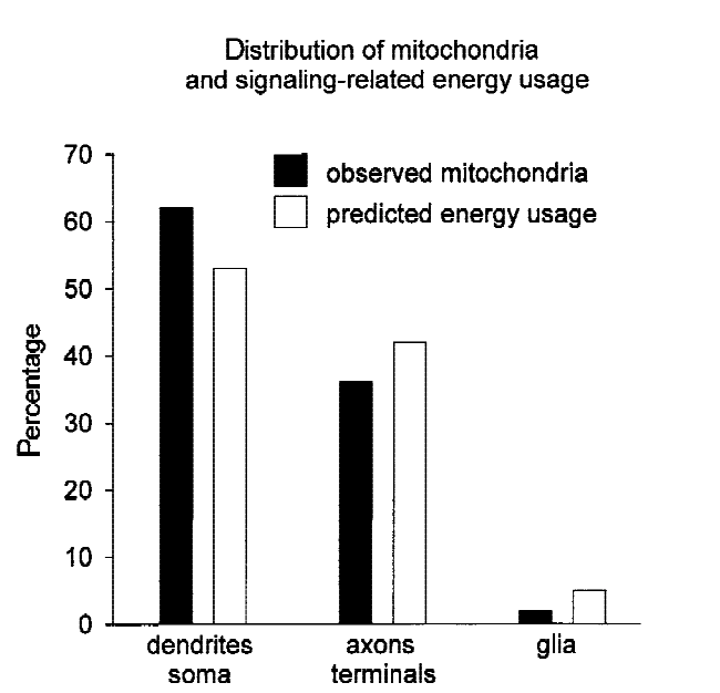
Overall, while some experts are skeptical of the importance of glia to information-processing, the evidence that they play at least some role seems to me fairly strong.[378] From Open Philanthropy’s non-verbatim notes from a conversation with Prof. Anthony Zador: “Glia are very important to understanding disease, but Prof. Zador does not believe that they are important to computing in the brain” (p. 4). How central of a role, though, is a further question, and the total number of glial cells, together with their limited energy consumption relative to neurons, does not, to me, initially suggest that capturing this role would require substantially more FLOP/s than capturing standard neuron signaling and learning.
In addition to the chemical synapses involved in standard neuron signaling, neurons (and other cells) also form electrical synapses – that is, connections that allow ions and other molecules to flow directly from one cell into another. The channels mediating these connections are known as gap junctions.
These have different properties than chemical synapses. In particular:
- Electrical synapses are faster, passing signals in a fraction of a millisecond.[379] See Siegelbaum and Koester (2013d), (p. 178)
- Electrical synapses can be bi-directional, allowing each cell to influence the other.[380] See Siegelbaum and Koester (2013d), (p. 178)
- Electrical synapses allow graded transmission of sub-threshold electrical signals.[381] See Siegelbaum and Koester (2013d), (p. 178)
My impression is that electrical synapses receive much less attention in neuroscience than chemical synapses. This may be because they are thought to be some combination of:
- Much less common.[382]Siegelbaum and Koester (2013d): “Most synapses in the brain are chemical” (p. 177). Lodish et al. (2000): “We also briefly discuss electric synapses, which are much rarer, but simpler in function, than chemical synapses.” Purves et al. (2001): “Although they are a distinct … Continue reading
- More limited in the behavior they can produce (chemical synapses, for example, can amplify pre-synaptic signals).[383]Siegelbaum and Koester (2013d): “Electrical synapses are employed primarily to send rapid and stereotyped depolarizing signals. In contrast, chemical synapses are capable of more variable signaling and thus can produce more complex behaviors. They can mediate either excitatory or inhibitory … Continue reading
- Involved in synchronization between neurons, or global oscillation, that does not imply complex information-processing.[384]From Open Philanthropy’s non-verbatim notes from a conversation with Dr. Adam Marblestone: “Sometimes the coupling between neurons created by gap junctions is so fast that they are treated as one neuron for modeling purposes. Gap junctions are also often thought of as supporting some kind of … Continue reading
- Amenable to very simple modeling.[385]From Open Philanthropy’s non-verbatim notes from a conversation with Prof. Barak Pearlmutter: “[Prof. Pearlmutter] took the fact that gap junctions are roughly linear, and that they don’t involve time delays, as evidence they would be easy to model” (p. 3). Though Bullock et al. … Continue reading
Still, electrical synapses can play a role in task-performance,[386] Trenholm et al. (2013): “We identified a network of electrically coupled motion–coding neurons in mouse retina that act collectively to register the leading edges of moving objects at a nearly constant spatial location, regardless of their velocity” (abstract). and one expert suggested that they could create computationally expensive non-linear dynamics.[387]From Open Philanthropy’s non-verbatim notes from a conversation with Dr. Stephen Larson: “Dr. Larson thinks that gap junctions can contribute to non-linear dynamics and near-chaotic dynamics within neural networks. As a rough rule of thumb: the more non-linear a system is, the more … Continue reading What’s more, if they are sufficiently fast, or require sufficiently frequent updates, this could compensate for their low numbers. For example, one expert suggested that you can model gap junctions as synapses that update every timestep.[388] From Open Philanthropy’s non-verbatim notes from a conversation with Prof. Chris Eliasmith: “You can model a gap junction as a connection that updates every timestep, rather than every time a spike occurs” (p. 4). But if chemical synapses only receive spikes, and hence update, ~once per second, and we use 1 ms timesteps, you’d need to have ~1000x fewer gap junctions in order for their updates not to dominate.
Overall, my best guess is that incorporating electrical synapses would not substantially increase our FLOP/s budget, but this is centrally based on a sense that experts treat their role in information-processing as relatively minor.
Neuron activity creates local electric fields that can have effects on other neurons. These are known as ephaptic effects. We know that these effects can occur in vitro (see especially Chiang et al. (2019))[389]They show that a wave of periodic neural activity can propagate across two physically separated pieces of hippocampal tissue (separation that removes the possibility of chemical or electrical synaptic communication), and that this propagation was blocked by a mechanism that cancels the relevant … Continue reading and entrain action potential firing,[390]Anastassiou et al. (2011): “We found that extracellular fields induced ephaptically mediated changes in the somatic membrane potential that were less than 0.5 mV under subthreshold conditions. Despite their small size, these fields could strongly entrain action potentials, particularly for slow … Continue reading and Chiang et al. (2019) suggest that they may explain slow oscillations of neural activity observed in vivo.[391]Chiang et al. (2019): “Slow oscillations have been observed to propagate with speeds around 0.1 m s−1 throughout the cerebral cortex in vivo… The mechanism most consistent with the data is ephaptic coupling whereby a group of neurons generates an electric field capable of activating the … Continue reading
A recent paper, though, suggests that the question of whether they have any functional relevance in vivo remains quite open,[392]Anastassiou and Koch (2015): “The biggest question about ephaptic coupling to endogenous fields remains its functional role: does such nonsynaptic, electric communication contribute to neural function and computationsin the healthy brain (e.g., in the absence of the strong fields generated during … Continue reading and one expert thought them unlikely to be important to task-performance.[393] From Open Philanthropy’s non-verbatim notes from a conversation with Prof. Anthony Zador: “Prof. Zador believes that ephaptic communication is very unlikely to be important to the brain’s information-processing” (p. 4).
One reason for doubt is that the effects on neuron membrane potential appear to be fairly small (e.g., <0.5 mV, compared with the ~15 mV gap between resting membrane potential and the threshold for firing),[394] Resting membrane potential is typically around -70 mV, and the threshold for firing is around -55 mV, though these vary somewhat. Anastassiou and Koch (2015): “such effects are likely to be small (e.g., compared to spike threshold)” (see “Outlook”). and may be drowned out by noise artificially lacking in vitro.[395]Anastassiou and Koch (2015): “The usefulness of such studies for understanding ephaptic coupling to endogenous fields is limited–chiefly, the cases emulated in slice oversimplify in vivo activity where neurons are continuously bombarded by hundreds of postsynaptic currents along their … Continue reading
Even if they were task-relevant, though, they would be spatially imprecise – arising from, and exerting effects on, the activity of groups of neurons, rather than on individual cells. Two experts took this as reason to think their role in task-performance would not be computationally expensive to capture.[396]From Open Philanthropy’s non-verbatim notes from a conversation with Prof. Anthony Zador: “Prof. Zador believes that ephaptic communication is very unlikely to be important to the brain’s information-processing. Even if it was important, though, it would be a form of global signaling, and so … Continue reading That said, actually modeling electric fields seems plausibly quite FLOP/s-intensive.[397]Sandberg and Bostrom (2008)): “If ephaptic effects were important, the emulation would need to take the locally induced electromagnetic fields into account. This would plausibly involve dividing the extracellular space (possibly also the intracellular space) into finite elements where the field … Continue reading
Action potentials are traditionally thought of as binary choices – a neuron fires, or it doesn’t – induced by changes to somatic membrane potential, and synaptic transmission as a product of this binary choice.[398]Bullock et al. (2005), describing the history of early neuroscience: “physiological studies established that conduction of electrical activity along the neuronal axon involved brief, all-or-nothing, propagated changes in membrane potential called action poten- tials. It was thus often assumed … Continue reading But in some contexts, this is too simple. For example:
- The waveform of an action potential (that is, its amplitude and duration) can vary in a way that affects neurotransmitter release.[399]Zbili and Debanne (2019): “When it invades the presynaptic terminal, the spike provokes the opening of voltage-gated calcium channels (Cav), leading to an increase of Ca2+concentration in the bouton and the release of neurotransmitters. Due to the power law between intra-terminal … Continue reading
- Variations in the membrane potential that occur below the threshold of firing (“subthreshold” variations) can also influence synaptic transmission.[400]Zbili and Debanne (2019): “the synaptic strength depends on the subthreshold membrane potential of the presynaptic cell, indicating that the presynaptic spike transmits this analog information to the postsynaptic cell. However, the direction of this modulation of synaptic transmission seems to … Continue reading
- Certain neurons – for example, neurons in early sensory systems,[401]Juusola et al. (1996): “Many neurons use graded membrane-potential changes, instead of action potentials, to transmit information. Traditional synaptic models feature discontinuous transmitter release by presynaptic action potentials, but this is not true for synapses between graded-potential … Continue reading and neurons in invertebrates[402]Graubard et al. (1980): “Graded synaptic transmission occurs between spiking neurons of the lobster stomatogastric ganglion. In addition to eliciting spike-evoked inhibitory potentials in postsynaptic cells, these neurons also release functionally significant amounts of transmitter below the … Continue reading – also release neurotransmitter continually, in amounts that depend on non-spike changes to pre-synaptic membrane potential.[403]Graded synaptic transmission is distinct from the spontaneous release of neurotransmitter associated with what are called “miniature postsynaptic currents.” From Faisal et al. (2008): “The classic manifestation of synaptic noise is the spontaneous miniature postsynaptic current (mPSC) that … Continue reading
- Some in vitro evidence suggests that action potentials can arise in axons without input from the soma or dendrites.[404]See Dugladze et al. (2012): “We found that during in vitro gamma oscillations, ectopic action potentials are generated at high frequency in the distal axon of pyramidal cells (PCs) but do not invade the soma. At the same time, axo-axonic cells (AACs) discharged at a high rate and tonically … Continue reading
Do these imply substantial increases to FLOP/s budgets? Most of the studies I looked at seemed to be more in the vein of “here is an effect that can be created in vitro” than “here is a widespread effect relevant to in vivo task-performance,” but I only looked into this very briefly, the possible mechanisms/complexities are diverse, and evidence of the latter type is rare regardless.
Some effects (though not all)[405]Pre-synaptic hyperpolarization (decreasing the membrane potential) can have effects within 15-50 ms. Zbili and Debanne (2019): “ADFs present various time constants which determine their potential roles in network physiology. In fact, in most of the studies, d-ADF needs 100 ms to several … Continue reading also required sustained stimulation (e.g., “hundreds of spikes over several minutes,”[406] Sheffield (2011): “In a subset of rodent hippocampal and neocortical interneurons, hundreds of spikes, evoked over minutes, resulted in persistent firing that lasted for a similar duration” (abstract). or “100 ms to several seconds of somatic depolarization”[407] Zbili and Debanne (2019) report that in most studies, it takes “100 ms to several seconds of presynaptic depolarization” (p. 8). ); and the range of neurons that can support axon signaling via sub-threshold membrane potential fluctuations also appears somewhat unclear, as the impact of such fluctuations is limited by the voltage decay along the axon.[408]My understanding is that the applicability of this consideration depends on the “length” or “space” constant associated with different axons in the brain, where the relevant issue is that the influence of pre-synaptic membrane potential changes along the axon decays exponentially in absence … Continue reading
Overall, though, I don’t feel very informed or clear about this one. As with electrical synapses, I think the central consideration for me is that the field doesn’t seem to treat it as central.
Blood flow in the brain correlates with neural activity (this is why fMRI works). This is often explained via the blood’s role in maintaining brain function (e.g., supplying energy, removing waste, regulating temperature).[409] Moore and Cao (2008): “The standard modern view of blood flow is that it serves a physiological function unrelated to information processing, such as bringing oxygen to active neurons, eliminating “waste” generated by neural activity, or regulating temperature” (p. 2035). Moore and Cao (2008)), though, suggest that blood flow could play an information-processing role as well – for example, by delivering diffusible messengers like nitric oxide, altering the shape of neuron membranes, modulating synaptic transmission by changing brain temperatures, and interacting with neurons indirectly via astrocytes.[410] See Moore and Cao (2008), (p. 2037-2040). The timescales of activity-dependent changes in blood flow are on the order of hundreds of milliseconds (the effects of such changes often persist after a stimulus has ended, but Moore and Cao believe this is consistent with their hypothesis).[411]Moore and Cao (2008): “the somatosensory neocortex, blood flow increases measured using laser Doppler have been observed <200 ms after the onset of sensory-evoked neural responses (Matsuura et al. (1999); Norup Nielsen and Lauritzen (2001)). Similarly, optical imaging techniques that … Continue reading
My impression, though, is that most experts don’t think that blood flow plays a very direct or central role in information-processing.[412]From Open Philanthropy’s non-verbatim notes from a conversation with Dr. Stephen Larson: “It’s generally thought that blood flow is more of an epiphenomenon/a sign that other forms of information processing are occurring (akin to the heat generated by a CPU), than a mechanism of … Continue reading And the spatial resolution appears fairly coarse regardless: Moore and Cao (2008) suggest resolution at the level of a cortical column (a group of neurons[413] The exact number, along with the definition of a column, appears to be the subject of some debate (see Rakic (2008) for complaints). Krueger (2008): “In humans, each column contains 1000 to 10,000 cells.” ), or an olfactory glomerulus (a cluster of connections between cells).[414]Moore and Cao (2008): “In the somatosensory and visual neocortex, a general consensus exists that the pattern of increased blood flow is similar to that of subthreshold neural activity, with a peak in signal that is localized to a cortical column (400 m) and an extent spanning several columns … Continue reading
Overall FLOP/s for other signaling mechanisms
Here is a chart summarizing some of the considerations just canvassed (see the actual sections for citations).
| MECHANISM | DESCRIPTION | SPEED | SPATIAL PRECISION | NUMBER/FREQUENCY | EVIDENCE FOR TASK-RELEVANCE |
|---|---|---|---|---|---|
| Other chemical signals | Chemical signals other than classical neurotransmitters. Includes neuropeptides, gases like nitrous oxide, endocannabinoids, and others. | Limited by the speed of chemical diffusion, and by the timescales of metabotropic receptors. | Imprecise. Affect groups of cells by diffusing through the extracellular space and/or through cell membranes, rather than via synapses. | Very common. However, some signal broadcasts are fairly rare, and may take ~400 spikes to trigger. | Strong. Can alter circuit dynamics and neuron input-output functions, role in synaptic plasticity. |
| Glia | Non-neuron cells traditionally thought to play a supporting role in the brain, but some of which may be more directly involved in task-performance. | Some local calcium responses within ~100 ms; other calcium signaling on timescales of seconds or longer. | Can respond locally to individual synaptic events. | ~1:1 ratio with neurons (not 100:1). Astrocytes (the most clearly task-relevant type of glial cell) are only 20-40% of glia. | Moderate. Role in zebrafish behavior. Plausible role in plasticity, synaptic transmission, and elsewhere. However, glia have a much smaller energy budget than neurons. |
| Electrical synapses | Connections between cells that allow ions and other molecules to flow directly from one to the other. | Very fast. Can pass signals in a fraction of a millisecond. | Precise. Signals are passed between two specific cells. But may function to synchronize groups of neurons. | Thought to be less common than chemical synapses (but may be passing signals more continuously, and/or require more frequent updates?). | Can play a role, but thought to be less important than chemical synapses? More limited range of signaling behaviors. |
| Ephaptic effects | Local electrical fields that can impact neighboring neurons. | ? Some oscillations that ephaptic effects could explain are slow-moving. Unsure about speed of lower-level effects. | Imprecise. Arises from activity of many cells, effects not targeted to specific cells. | ? | Weak? Small effects on membrane potential possibly swamped by noise in vivo. |
| Other forms of axon signaling | Processes in a neuron other than a binary firing decision that impact synaptic transmission. | ? Some effects required sustained stimulation (minutes of spiking, 100 ms to seconds of depolarization). Others arose more quickly (15-50 ms of hyperpolarization). | Precise, proceeds via axons/individual synapses. | Unclear what range of neurons can support some of the effects (e.g., sub-threshold influences on synaptic transmission). | Some effects relevant in at least some species/contexts. Other evidence mostly from in vitro studies? |
| Blood flow | Some hypothesize that blood flow in the brain is involved in information-processing. | Responses within hundreds of ms, which persist after stimulus has ended. | Imprecise. At the level of a cortical column, or a cluster of connections between cells. | ? | Weak. Widely thought to be epiphenomenal. |
Still, as mentioned earlier, my best guess is that capturing the role of other signaling mechanisms (known and unknown) in task-performance does not require substantially more FLOP/s than capturing standard neuron signaling and learning. This guess is primarily grounded in a sense that computational neuroscientists generally treat standard neuron signaling (and the plasticity thereof) as the primary vehicle of information-processing in the brain, and other mechanisms as secondary.[417] A number of experts we engaged with indicated that many computational neuroscientists would not emphasize other mechanisms very much (though their comments in this respect are not publicly documented); and the experts I interviewed didn’t tend to emphasize such mechanisms either. An initial look at the speed, spatial precision, prevalence, and task-relevance of the most salient of these mechanisms seems compatible with such a stance, so I’m inclined to defer to it, despite the possibility that it emerges primarily from outdated assumptions and/or experimental limitations, rather than good evidence.
Overall mechanistic method FLOP/s
Here are the main numbers we’ve discussed thus far:
Standard neuron signaling: ~1e13-1e17 FLOP/s
Synaptic transmission: 1e13-1e17 FLOP/s
Spikes through synapse per second: 1e13-1e15
FLOPs per spike through synapse:Low: 1 (one addition and/or multiply operation, reflecting impact on post-synaptic membrane potential)
High: 100 (covers 40 FLOPs for synaptic conductances, plus cushion for other complexities)
Firing decisions: 1e13-1e17 FLOP/s
Number of neurons: 1e11
FLOP/s per neuron:
Low: 100 (ReLU, 10 ms timesteps)
Middle: 10,000 (Izhikevich model, 1 ms timesteps)
High: 1,000,000 (single compartment Hodgkin-Huxley model, 0.1 ms timesteps)
Learning: <1e13 – 1e17 FLOP/s
Spikes through synapse per second: 1e13-1e15
FLOPs per spike through synapse:
Low: <1 (possibly due to slow timescales)
Middle: 1-10 (covers various learning models – Hebbian plasticity, first-order gradient methods, possibly Benna and Fusi (2016) – and expert estimates, relative to low end baselines)
High: 100 (covers those models with more cushion/relative to higher baselines).
Other signaling mechanisms: do not meaningfully increase the estimates above.Overall range: ~1e13-1e17 FLOP/s[418] Technically, this would be ~3e13-3e17 FLOP/s, if we were really adding up synaptic transmission, firing decisions, and learning. But these ranges are sufficiently made-up and arbitrary that this sort of calculation seems to me misleadingly precise.
To be clear: the choices of “low” and “high” here are neither principled nor fully independent, and I’ve rounded aggressively.[419]That is, I did not do fully independent analyses of each of these areas and then combine them (this is why the ranges are so similar). Rather, I started with a baseline, default model of 1 FLOP per spike through synapse, and then noted that budgeting 10-100x of cushion on top of that would cover … Continue reading Indeed, another, possibly more accurate way to summarize the estimate might be:
“There are roughly 1e14-1e15 synapses in the brain, receiving spikes about 0.1-1 times a second. A simple estimate budgets 1 FLOP per spike through synapse, and two extra orders of magnitude would cover some complexities related to synaptic transmission, as well as some models of learning. This suggests something like 1e13-1e17 FLOP/s. You’d also need to cover firing decisions, but various simple neuron models, scaled up by 1e11 neurons, fall into this range as well, and the high end (1e17 FLOP/s) would cover a level of modeling detail that I expect many computational neuroscientists to think unnecessary (single compartment Hodgkin-Huxley). Accounting for the role of other signaling mechanisms probably doesn’t make much of a difference to these numbers.”
That is, this is meant to be a plausible ballpark, covering various types of models that seem plausibly adequate to me.
Here are some ways it could be too low:
- The choice to budget FLOP/s for synaptic transmission and learning based on spikes through synapses, rather than timesteps at synapses, is doing a lot of work. If we instead budgeted based on timesteps, and used something like 1 ms resolution, we’d start with 1e17-1e18 FLOP/s as a baseline (1 FLOP per timestep per synapse). Finer temporal resolutions, and larger numbers of FLOPs per time-step, would drive these numbers higher.
- Some neural processes are extremely temporally precise. For example, neurons in the owl auditory system can detect auditory stimulus timing at a precision of less than ten microseconds.[420]Funabiki et al. (2011): “In owls, NL neurons change their firing rates with changes in ITD of <10 μs (Carr and Konishi (1990); Peña et al. (1996)), far below the spike duration of the neurons (e.g., ∼1 ms). The data used for modeling these coincidence detection processes have so far come … Continue reading These cases may be sufficiently rare, or require combining a sufficient number of less-precise inputs, that they wouldn’t make much of a difference to the overall budget. However, if they are indicative of a need for much finer temporal precision across the board, they could imply large increases.
- Dendritic computation might imply much larger FLOP/s budgets than single-compartment Hodgkin-Huxley models.[421]From Open Philanthropy’s non-verbatim notes from a conversation with Prof. Eric Jonas: “Active dendritic computation could conceivably imply something like 1-5 orders of magnitude more compute than a simple linear summation model of a neuron. And if dendritic morphology is evolving over time, … Continue reading Results like Beniaguev et al. (2020) (~1e10 FLOP/s per neuron), discussed above, seem like some initial evidence for this.
- Some CNN/RNN models used to predict the activity of retinal neurons are very FLOP/s intensive as well. I discuss this in Section 3.1.
- Complex molecular machinery at synapses or inside neurons might implement learning algorithms that would require more than 100 FLOPs per spike through synapse to replicate.[422] See e.g. Bhalla (2014). And I am intrigued by theoretical results showing that various models of synaptic plasticity lead to problems like catastrophic forgetting, and that introducing larger numbers of dynamical variables at synapses might help with online learning.[423]Kaplanis et al. (2018): “we show that by equipping tabular and deep reinforcement learning agents with a synaptic model that incorporates this biological complexity (Benna and Fusi (2016)), catastrophic forgetting can be mitigated at multiple timescales. In particular, we find that as well as … Continue reading
- One or more of the other signaling mechanisms in the brain might introduce substantially additional FLOP/s burdens (neuromodulation and glia seem like prominent candidates, though I feel most uncertainty about the specific arguments re: gap junctions and alternative forms of axon signaling).
- Processes in the brain that take place over longer timescales involve interactions between many biophysical variables in the brain that are not normally included in e.g. simple models of spiking. The length of these timescales might limit the compute burdens such interactions imply, but if not, updating all relevant variables at a frequency similar to the most frequently updated variables could imply much larger compute burdens.[424]From Open Philanthropy’s non-verbatim notes from a conversation with Prof. Eve Marder: “In reality, the nervous system has an incredible ability to move seamlessly between timescales ranging from milliseconds to years, and the relevant processes interact. That is, short time-scale processes … Continue reading
- Some of the basic parameters I’ve used could be too low. The average spike rate might be more like 10 Hz than 0.1-1 Hz (I really doubt 100 Hz); synapse count might be >1e15; Hodgkin-Huxley models might require more FLOP/s than Izhikevich (2004) budgets, etc. Indeed, I’ve been surprised at how uncertain many very basic facts about the brain appear to be, and how wrong previous widely-cited numbers have been (for example, a 10:1 ratio between glia and neurons was widely accepted until it was corrected to roughly 1:1).[425] See von Bartheld et al. (2016): “The recently validated isotropic fractionator demonstrates a glia:neuron ratio of less than 1:1… We review how the claim of one trillion glial cells originated, was perpetuated, and eventually refuted.” (p. 1)).
There are also broader considerations that could incline us towards higher numbers by default, and/or skepticism of arguments in favor of the adequacy of simple models:
- We might expect evolution to take advantage of every possible mechanism and opportunity available for increasing the speed, efficiency, and sophistication of its information-processing.[426]From Open Philanthropy’s non-verbatim notes from a conversation with Prof. Erik De Schutter: “The brain was not engineered. Rather, it evolved, and evolution works by adding complexity, rather than by simplification… Indeed, in general, many scientists who approach the brain from an … Continue reading Some forms of computation in biological systems, for example, appear to be extremely energy efficient.[427]See e.g. Kempes et al. (2017): “Here we show that the computational efficiency of translation, defined as free energy expended per amino acid operation, outperforms the best supercomputers by several orders of magnitude, and is only about an order of magnitude worse than the Landauer bound” … Continue reading Indeed, I think that further examination of the sophistication of biological computation in other contexts could well shift my default expectations about the brain’s sophistication substantially (though I have tried to incorporate hazy forecasts in this respect into my current overall view).[428]See e.g. from Open Philanthropy’s non-verbatim notes from a conversation with Prof. Eric Jonas: “Various discoveries in biology have altered Prof. Jonas’s sense of the complexity of what biological systems can be doing. Examples in this respect include non-coding RNA, the complexity present … Continue reading
- It seems possible that the task-relevant causal-structure of the brain’s biology is just intrinsically ill-suited to replication using digital computer hardware, even once you allow for whatever computational simplifications are available (though neuromorphic hardware might do better). For example, the brain may draw on analog physical primitives,[429]Sarpeshkar (1998): “Items 1 through 3 show that analog computation can be far more efficient than digital computation because of analog computation’s repertoire of rich primitives. For example, addition of two parallel 8-bit numbers takes one wire in analog circuits (using Kirchoff’s current … Continue reading continuous (or very fine-grained) temporal dynamics,[430] See e.g. Open Philanthropy’s non-verbatim notes from a conversation with Prof. Eve Marder: “Unlike digital computers, the brain integrates over very long timescales at very fast speeds easily and seamlessly” (p. 3). and/or complex biochemical interactions that are cheap for the brain, but very expensive to simulate.[431]From Open Philanthropy’s non-verbatim notes from a conversation with Prof. Rosa Cao: “Digital computers achieve speed and reliability by ignoring many dimensions of what is happening in the system. In such a context, you only care about whether the voltage in the transistors is above or below … Continue reading
- Limitations on tools and available data plausibly do much to explain the concepts and assumptions most prominent in neuroscience. As these limitations loosen, we may identify much more complex forms of information-processing than the field currently focuses on.[432]From Open Philanthropy’s non-verbatim notes from a conversation with Dr. Adam Marblestone: “Neuroscience is extremely limited by available tools. For example, we have the concept of a post-synaptic potential because we can patch-clamp the post-synaptic neuron and see a change in voltage. When … Continue reading Indeed, it might be possible to extrapolate from trends in this vein, either in neuroscience or across biology more broadly.[433] Thanks to Luke Muehlhauser for suggesting this possibility.
- Various experts mentioned track-records of over-optimism about the ease of progress in biology, including via computational modeling;[434]From Open Philanthropy’s non-verbatim notes from a conversation with Prof. Eric Jonas: “There is a history of over-optimism about scientific progress in neuroscience and related fields. Prof. Jonas grew up in an era of hype about progress in science (e.g., “all of biology will yield its … Continue reading overly-aggressive claims in favor of particular neuroscientific research programs;[435]From Open Philanthropy’s non-verbatim notes from a conversation with Prof. Eric Jonas: “many in the neuroscience community feel that some neuroscientists made overly aggressive claims in the past about what amount of progress in neuroscience to expect (for example, from simulating networks of … Continue reading and over-eagerness to think of the brain via in terms of the currently-most-trendy computational/technological paradigms.[436]From Open Philanthropy’s non-verbatim notes from a conversation with Prof. Eric Jonas: “[Prof. Jonas] also has a long-term prior that researchers are too quick to believe that the brain is doing whatever is currently popular in machine learning, and he doesn’t think we’ve found the right … Continue reading To the extent such track records exist, they could inform skepticism about arguments and expert opinions in a similar reference class (though on their own, they seem like only very indirect support for very large FLOP/s requirements, as many other explanations of such track records are available).
And of course, more basic paradigm mistakes are possible as well.[437]Two experts thought this unlikely. From Open Philanthropy’s non-verbatim notes from a conversation with Dr. Adam Marblestone: “Dr. Marblestone thinks that the probability that the field of neuroscience rests on some very fundamental paradigm mistake is very low. We’re missing a unified … Continue reading
This is a long list of routes to higher numbers; perhaps, then, we might expect at least one of them to track the truth. However:
- Some particular routes are correlated: for example, worlds in which the brain can implement very sophisticated, un-simplifiable computation at synapses seem more likely to be ones in which it can implement such computation within dendrites as well.[438] Thanks to Dr. Dario Amodei and Dr. Owain Evans for suggesting that I consider correlations between different routes to higher numbers.
- My vague impression is that experts tend to be inclined towards simplification vs. complexity across the board, rather than in specific patterns that differ widely. If this is true, then the reliability of the assumptions and methods these experts employ might be a source of broader correlations.
- Some of these routes are counterbalanced by corresponding routes to lower numbers (e.g., basic parameters could be too high as well as too low; relevant timescales could be more coarse-grained rather than more fine-grained; etc). And there are more general routes to lower numbers as well, which would apply even if some of the considerations surveyed above are sound (see next section).
Here are a number of ways 1e13-1e17 FLOP/s might be overkill (I’ll focus, here, on ways that are actively suggested by examination of the brain’s mechanisms, rather than on the generic consideration that for any given way of performing a task, there may be a more efficient way).
Neuron populations and manifolds
The framework above focuses on individual neurons and synapses. But this could be too fine-grained. For example, various popular models in neuroscience involve averaging over groups of neurons, and/or treating them as redundant representations of high-level variables.[439]From Open Philanthropy’s non-verbatim notes from a conversation with Prof. Markus Meister: “Synapses are noisy, and silicon isn’t; and the brain uses huge numbers of neurons to represent the same variable, probably because a single neuron can’t do it robustly. Prof. Meister expects that … Continue reading
Indeed, in vivo recording shows that the dimensionality of the activity of a network of neurons is much smaller than the number of neurons themselves (Wärnberg and Kumar (2017) suggest a subspace spanned by ~10 variables, for local networks consisting of thousands of neurons).[440]From the author summary: “A network in the brain consists of thousands of neurons. A priori, we expect that the network will have as many degrees of freedom as its number of neurons. Surprisingly, experimental evidence suggests that local brain activity is confined to a subspace spanned by ~10 … Continue reading This kind of low-dimensional subspace is known as a “neural manifold.”[441] My thanks to the expert who suggested I consider this.
Some of this redundancy may be about noise: neurons are unreliable elements, so representing high-level variables using groups of them may be more robust.[442]Faisal et al. (2008): “Averaging is used in many neural systems in which information is encoded as patterns of activity across a population of neurons that all subserve a similar function (for example, see REFS 142,143): these are termed neural population codes. A distributed representation of … Continue reading Digital computers, though, are noise-free.
In general, the possibility of averaging over or summarizing groups of neurons suggests smaller budgets than the estimates above – possibly much smaller. If I had more time for this project, this would be on the top of my list for further investigation.
Transistors and emulation costs
If we imagine applying the mechanistic method to a digital computer we don’t understand, we plausibly end up estimating the FLOP/s required to model the activity of very low-level components: e.g. transistors, logic gates, etc (or worse, to simulate low-level physical processes within transistors). This is much more than the FLOP/s the computer can actually perform.
For example: a V100 has about 2e10 transistors, and a clock speed of ~1e9 Hz.[443] See p. 10 here. A naive mechanistic method estimate for a V100 then, might budget 1 FLOP per clock-tick per transistor: 2e19 FLOP/s. But the chip’s actual computational capacity is ~1e14 FLOP/s – a factor of 2e5 less.
The costs of emulating different computer systems at different levels of detail may also be instructive here. For example, one attempt to simulate a 6502 microprocessor (original clock speed of ~1 Mhz) at the transistor level managed to run the simulated chip at 1 Khz using a computer running at ~1 GHz, suggesting a factor of ~1e6 slow-down.[444] From here: “Michael Steil and some collaborators had ported the code to C and were able to run at about 1kHz… This was only a thousand times slower than the original, running on a computer that was perhaps two million times faster.” Other emulations may be more efficient.
Of course, there is no easy mapping between computer components and brain components; and there are components in the brain at lower-levels than neurons (e.g., ion channels, proteins, etc). Still, applying the mechanistic method to digital computers suggests that when we don’t know how the system works, there is no guarantee that we land on right level of abstraction, and hence that estimates based on counting synapses, spikes, etc. could easily be overkill relative to the FLOP/s requirements of the tasks the brain can actually perform (I discuss this issue more in the appendix).
How much overkill is harder to say, at least using the mechanistic method alone: absent knowledge of how a V100 processes information, it’s not clear to me how to modify the mechanistic method to arrive at 1e14 FLOP/s rather than 2e19. Other methods might do better.
Note, though, that applying the mechanistic method without a clear understanding of whether models at the relevant level of abstraction could replicate task-performance at all could easily be “underkill” as well.
Do we need the whole brain?
Do we need the whole brain? For some tasks, no. People with parts of their brains missing/removed can still do various things.
A dramatic example is the cerebellum, which contains ~69 billion neurons – ~80% of the neurons in the brain as a whole.[445] Dr. Dario Amodei suggests considering whether we can leave out the cerebellum for certain types of tasks. Some people (a very small number) don’t have cerebellums. Yet there are reports that in some cases, their intelligence is affected only mildly, if at all (though motor control can also be damaged, and some cognitive impairment can be severe).[446]From the National Organization for Rare Disorders: “Additional reports have noted individuals with cerebellar agenesis whose mental capacities were unaffected and who did not exhibit any symptoms of cerebellar agenesis (asymptomatic cases). However, other researchers have disputed these claims, … Continue reading
Does this mean we can reduce our FLOP/s budget by 80%? I’m skeptical. For one thing, while the cerebellum accounts for a large percentage of the brain’s neurons, it appears to account for a much smaller percentage of other things, including volume (~10%),[447] Swanson (1995) (p. 473). mass (~10%),[448] Azevedo et al. (2009) (p. 536), suggests that the cerebellum weights ~154.02 g (10.3% of the brain’s mass), whereas the cerebral cortex weighs 1232.93 g (81.8% of the brain’s mass). energy consumption (<10%),[449]I’m basing this on the fact that the cerebellum is ~10% of the brain’s weight, relative to ~80% for the cortex, and Howarth et al’s (2012) suggestion that energy consumption per gram is higher in the cerebral cortex than in the cerebellar cortex: “Including this range of values would result … Continue reading and maybe synapses (and synaptic activity dominates many versions of the estimates above).[450]Most of the neurons in the cerebellum (specifically, about 50 billion, at least according to Llinás et al. (2004) (p. 277)) are cerebellar granule cells, which appear to have a comparatively small number of synapses each: “[Granule] cells are the most numerous in the CNS; there are about 5 × … Continue reading
More importantly, though, we’re looking for FLOP/s estimates that apply to the full range of tasks that the brain can perform, and it seems very plausible to me that some of these tasks (neurosurgery? calligraphy?) will rely crucially on the cerebellum. Indeed, the various impairments generally suffered by patients without cerebellums seem suggestive of this.
This last consideration applies across the board, including to other cases in which various types of cognitive function persist in the face of missing parts of the brain,[451]For example, Pulsifer et al. (2004) report that in a study of 71 patients who underwent hemispherectomy for severe and intractable seizures, “Cognitive measures typically changed little between surgery and follow-up, with IQ change <15 points for 34 of 53 patients” (abstract) (though … Continue reading neuron/synapse loss,[452]Glancing at one study, asymptomatic Alzehimer’s disease does not appear to be associated with neuron loss. See Andrade-Moraes et al. (2013): “We found a great reduction of neuronal numbers in the hippocampus and cerebral cortex of demented patients with Alzheimer’s disease, but not in … Continue reading etc. That is, while I expect it to be true of many tasks (perhaps even tasks important to AI developers, like natural language processing, scientific reasoning, social modeling, etc.) that you don’t need the whole brain to do them, I also expect us to be able to construct tasks that do require most of the brain. It also seems very surprising, from an evolutionary perspective, if large, resource-intensive chunks of the brain are strictly unnecessary. And the reductions at stake seem unlikely to make an order-of-magnitude difference anyway.
Constraints faced by evolution
In designing the brain, evolution faced many constraints less applicable to human designers.[453] Dr. Dario Amodei suggested considering these constraints. See also the citations throughout the rest of the section. For example, constraints on:
- The brain’s volume.
- The brain’s energy consumption.
- The growth and maintenance it has to perform.[454]Sandberg (2016): “Biology has many advantages in robustness and versatility, not to mention energy efficiency. Nevertheless, it is also fundamentally limited by what can be built out of cells with a particular kind of metabolism, the fact that organisms need to build themselves from the inside, … Continue reading
- The size of the genome it has to be encoded in.[455]See Moravec (1988): “There is insufficient information in the 1010 bits of the human genome to custom-wire many of the 1014 synapses in the brain” (p. 166). See also Zador (2019): “ The human genome has about 3 × 10⁹ nucleotides, so it can encode no more than about 1 GB of … Continue reading
- The comparatively slow and unreliable elements it has to work with.[456]Moravec (1988): “The slow switching speed and limited signaling accuracy of neurons rules out certain solutions for neural circuitry that are easy for computers” (p. 165). Dmitri Strukov’s comments here: “we should also keep in mind that over millions of years the evolution of biological … Continue reading
- Ability to redesign the system from scratch.[457]Moravec (1988): “The neuron’s basic information-passing mechanism – the release of chemicals that affect the outer membranes of other cells – seems to be a very primitive one that can be observed in even the simplest free-swimming bacteria. Animals seem to be stuck with this arrangement … Continue reading
It may be that these constraints explain the brain’s functional organization at sufficiently high-levels that if we understood the overarching principles at work, we would see that much of what the brain does (even internally) is comparatively easy to do with human computers, which can be faster, bigger, more reliable, more energy-intensive, re-designed from scratch, and built using external machines on the basis of designs stored using much larger amounts memory.[458]Here, the distinction between “finding ways to do it the way the brain does it, but with a high-level of simplification/increased efficiency” and “doing it some other way entirely” is blurry. I have the former vaguely in mind, but see the appendix for more detailed discussion. See … Continue reading This, too, suggests smaller budgets.
Beyond the mechanistic method
Overall, I find the considerations pointing to the adequacy of smaller budgets more compelling than the considerations pointing to the necessity of larger ones (though it also seems, in general, easier to show that X is enough, than that X is strictly required – an asymmetry present throughout the report). But the uncertainties in either direction rightly prompt dissatisfaction with the mechanistic method’s robustness. Is there a better approach?
The functional method
Let’s turn to the functional method, which attempts to identify a portion of the brain whose function we can already approximate with artificial systems, together with the computational costs of doing so, and then to scale up to an estimate for the brain as a whole.
Various attempts at this method have been made. To limit the scope of the section, I’m going to focus on two categories: estimates based on the retina, and estimates based on the visual cortex. But I expect many problems to generalize.
As a preview of my conclusion: I give less weight to these estimates than to the mechanistic method, primarily due to uncertainties about (a) what the relevant portion of the brain is doing (in the case of the visual cortex), (b) differences between that portion and the rest of the brain (in the case of the retina), and (c) the FLOP/s required to fully replicate the functions in question. However, I take visual cortex estimates as some weak evidence that the mechanistic method range above (1e13-1e17 FLOP/s) isn’t much too low. Some estimates based on recent deep neural network models of retinal neurons point to higher numbers. I take these on their own as even weaker evidence, but I think they’re worth understanding better.
The retina
As I discussed in Section 2.1.2.1.2, the retina is one of the best-understood neural circuits.[459]From Open Philanthropy’s non-verbatim notes from a conversation with Prof. Markus Meister: “The computations performed in the retina are fairly well-understood. There is more to learn, of course, but the core framework is in place. We have a standard model of the retina that can account for a … Continue reading Could it serve as a basis for a functional method estimate?
We don’t yet have very good artificial retinas (though development efforts are ongoing).[460]See Yue et al. (2016) for a review of progress in retinal implant development as of 2016. From the Stanford Artificial Retina Project: “The current state of the art of retinal prostheses can be summed up as such: no blind patient today would trade their cane or guide dog for a retinal … Continue reading However, this has a lot to do with engineering challenges – e.g., building devices that interface with the optic nerve in the right way.[461]From Open Philanthropy’s non-verbatim notes from a conversation with Prof. Markus Meister: “However, this lack of success is not about computation. People in the field generally agree that if you could make the right kind of one-to-one connection to the optic nerve fibers, you could compute … Continue reading Even absent fully functional artificial retinas, we may be able to estimate the FLOP/s required to replicate retinal computation.
Moravec (1988, 1998, and 2008) offers some estimates in this vein.[462] See Moravec (1988), Chapter 2 (p. 51-74). See also Moravec (1988) and Moravec (2008). Merkle (1989) uses a broadly similar methodology. He treats the retina as performing two types of operations – a “center surround” operation, akin to detecting an edge, and a “motion detection” operation – and reports that in his experience with robot vision, such operations take around 100 calculations to perform.[463]See Moravec (1988) (p. 57-60). For discussion of what a center-surround and a motion-detection operation in the retina consists in, see Meister et al. (2013): “A typical ganglion cell is sensitive to light in a compact region of the retina near the cell body, called the … Continue reading He then divides the visual field into patches, processing of which gets sent to a corresponding fiber of the optic nerve, and budgets ten edge/motion detection operations per patch per second (ten frames per second is roughly the frequency at which individual images become indistinguishable for humans).[464] See Moravec (1988) (p. 58-59). That said, he also acknowledges that “though separate frames cannot be distinguished faster than 10 per second, if the light flickers at the frame rate, the flicker itself is detectable until it reaches a frequency of about 50 flashes per second” (p. 59). This yields an overall estimate of:
1e6 ganglion cells × 100 calculations per edge/motion detection × 10 edge/motion detections per second = 1e9 calculations/sec for the whole retina
Is this right? At the least, it’s incomplete: neuroscientists have catalogued a wide variety of computations that occur in the retina, other than edge and motion detection (I’m not sure how many were known at the time). For example: the retina can anticipate motion,[465]See Gollisch and Meister (2010): “When the image of an object moves on the retina, it creates a wave of neural activity among the ganglion cells. One should expect that this wave lags behind the object image because of the delay in phototransduction. Instead, experiments show that the activity … Continue reading it can signal that a predicted stimulus is absent,[466]See Gollisch and Meister (2010): “A somewhat different form of anticipation can be observed when the visual system is exposed to a periodic stimulus, such as a regular series of flashes. The activated visual neurons typically become entrained into a periodic response. If the stimulus sequence is … Continue reading it can adapt to different lighting conditions,[467]Gollisch and Meister (2010): “Because the ambient light level varies over ~9 orders of magnitude in the course of a day, while spiking neurons have a dynamic range of only ~2 log units, the early visual system must adjust its sensitivity to the prevailing intensities. This adaptation to light … Continue reading and it can suppress vision during saccades.[468]Gollisch and Meister (2010): “During a saccade, the image sweeps across the retina violently for tens of milliseconds, precluding any useful visual processing. In humans, visual perception is largely suppressed during this period (Volkmann (1986); Burr et al. (1994); Castet and Masson (2000)). … Continue reading And further computations may await discovery.[469] Gollisch and Meister (2010): “The anatomical diversity suggests that there is much function left to be discovered and that we probably still have a good distance to go before understanding all the computations performed by the retina” (p. 14).
But since Moravec’s estimates, we’ve also made progress in modeling retinal computation. Can recent models provide better estimates?
Some of these models were included in Figure 7. Of these, it seems best to focus on models trained on naturalistic stimuli, retinal responses to which have proven more difficult to capture than responses to more artificial stimuli.[470]From Open Philanthropy’s non-verbatim notes from a conversation with Prof. Markus Meister: “It has taken more effort to simulate retinal responses to natural scenes than to artificial stimuli used in labs (e.g. spots, flashes, moving bars)” (p. 1). Heitman et al. (2016): “This paper tests … Continue reading RNN/CNN neural network models appear to have more success at this than some other variants,[471]See Figure 1C in Maheswaranathan et al. (2019), and Batty et al. (2017): “RNNs of varying architectures consistently outperformed LNs and GLMs in predicting neural spiking responses to a novel natural scene movie for both OFF and ON parasol retinal ganglion cells in both experiments (Figure … Continue reading so I’ll focus on two of these:
- Maheswaranathan et al. (2019), who train a three-layer CNN to predict the outputs of ganglion cells in response to naturalistic stimuli, and achieve a correlation coefficient greater than 0.7 (retinal reliability is 0.8).
- Batty et al. (2017), use a shared, two-layer RNN on a similar task, and capture around ~80% of explainable variance across experiments and cell types.
These models are not full replications of human retinal computation. Gaps include:
- Their accuracy can still be improved, and what’s missing might matter.[472]From Open Philanthropy’s non-verbatim notes from a conversation with Prof. E.J. Chichilnisky: “It’s hard to know when to stop fine-tuning the details of your model. A given model may be inaccurate to some extent, but we don’t know whether a given inaccuracy matters, or whether a human … Continue reading
- The models have only been trained on a very narrow class of stimuli.[473]From Open Philanthropy’s non-verbatim notes from a conversation with Dr. Stephen Baccus: “The visual system works under a wide range of conditions – for example, varying light levels and varying contrast levels. Experiments focused on a set of natural scenes only cover some subset of these … Continue reading
- Inputs are small (50 × 50 pixels or less) and black-and-white (though I think they only need to be as large as the relevant ganglion cell’s receptive field).
- These models don’t include adaptation, either (though one expert did not expect adaptation to make much of a difference to overall computational costs).[474]From Open Philanthropy’s non-verbatim notes from a conversation with Prof. Markus Meister: “The biochemistry involved in retinal light adaptation is well-understood, and it can be captured using a simplified computational model. Specifically, you can write down a three-variable dynamical model … Continue reading
- We probably need to capture correlations across cells, in addition to individual cell responses.[475]From Open Philanthropy’s non-verbatim notes from a conversation with Dr. Stephen Baccus: “These models focus on replicating the response of an individual retinal ganglion cell to a stimulus. However, it may also be necessary to replicate correlations between the responses of different cells in … Continue reading
- Maheswaranathan et al. (2019) use salamander retinal ganglion cells, results from which may not generalize well to humans (Batty et al. (2017) use primate cells, which seem better).[476]From Open Philanthropy’s non-verbatim notes from a conversation with Prof. E.J. Chichilnisky: “There is variability in retinal function both across species and between individuals of the same species. Mouse retinas are very different from human retinas (a difference that is often ignored), and … Continue reading
- There are a number of other possible gaps (see endnote).[477]For example, there are about 20 different types of retinal ganglion cells in humans (see Open Philanthropy’s non-verbatim notes from a conversation with Prof. E.J. Chichilnisky (p. 3)), which could vary in complexity. However, Prof. Stephen Baccus seemed to think that the data gathered … Continue reading
What sort of FLOP/s budgets would the above models imply, if they were adequate?
- The CNN in Maheswaranathan et al. (2019) requires about 2e10 FLOPs to predict the output of one ganglion cell over one second.[478]From Open Philanthropy’s non-verbatim notes from a conversation with Dr. Stephen Baccus: “Prof. Baccus and his colleagues have calculated that their CNN requires ~20 billion floating point operations to predict the output of one ganglion cell over one second (these numbers treat multiply and … Continue reading However, adding more ganglion cells only increases the costs in the last layer of the network. A typical experiment involves 5-15 cells, suggesting ~2e9 FLOP/s per cell, and one of the co-authors on the paper (Prof. Baccus) could easily imagine scaling up to 676 cells (the size of the last layer), which would cost ~20.4 billion FLOP/s (3e7 per cell); or 2500 cells (the size of the input), which would cost 22.4 billion FLOP/s (~1e7 per cell).[479]From Open Philanthropy’s non-verbatim notes from a conversation with Dr. Stephen Baccus: “Simulating more ganglion cells simultaneously only alters the last layer of the network, and so results in only a relatively small increase in computation. A typical experiment involves around 5-15 cells, … Continue reading I’ll use this last number, which suggests ~1e7 FLOP/s per retinal ganglion cell. However, I don’t feel that I have a clear grip on how to pick an appropriate number of cells.
- I estimate that the RNN in Batty et al. (2017) requires around 1e5 FLOP for one 0.83 ms bin.[480]My estimate is as follows. 1st layer: (31 × 31 (image patch) + 50 (inputs from previous time-step)) × 50 = 48,050 MACCs. Second layer: (50 feedforward inputs from layer 1 + 50 inputs from previous time-step) × 50 = 5,000 MACCs. Total MACCs per timestep: ~ 53,000. Multiplied by two for FLOPs vs. … Continue reading I’m less clear on how this scales per ganglion cell, so I’ll assume one cell for the whole network: e.g., ~1e8 FLOP/s per retinal ganglion cell.
These are much higher than Moravec’s estimate of 1000 calculations/s per ganglion cell, and they result in much higher estimates for the whole retina: 1e13 FLOP/s and 1e14 FLOP/s, respectively (assuming 1e6 ganglion cells).[481]Sarpeshkar (2010) estimates at least 1e10 FLOP/s for the retina, based on budgeting at least one floating-point multiplication operation per synapse, and a 12 Hz rate of computation (p. 749). However, he doesn’t (at least in that paragraph) say much to justify this assumption; and estimates that … Continue reading But it’s also a somewhat different task: that is, predicting retinal spike trains, as opposed to motion/edge detection more broadly.
Note, also, that in both cases, the FLOPs costs are dominated by the first layer of the network, which processes the input, so costs would scale with the size of the input (though the input size relevant to an individual ganglion cell will presumably be limited by the spatial extent of its receptive field).[482] From Open Philanthropy’s non-verbatim notes from a conversation with Dr. Stephen Baccus: “The largest amount of computation takes place in the first layer of the network. If the input size was larger, these numbers would scale up” (p. 6). And in general, the scale-up to the whole retina here is very uncertain, as I feel very uninformed about what it would actually look like to run versions of these models on such a scale (how much of the network could be reused for different cells, what size of receptive field each cell would need, etc).
What does it look like to scale up from these estimates to the brain as a whole? Here a few ways of doing so, and the results:
| BASIS FOR SCALING | ROUGH SCALING FACTOR | APPLIED TO: MORAVEC ESTIMATE (1E9 CALCS/S) | APPLIED TO:MAHESWARANATHAN ET AL. (2019)ESTIMATE (1E13 FLOP/S) | APPLIED TO: BATTY ET AL. (2019) ESTIMATE (1E14 FLOP/S) |
|---|---|---|---|---|
| Mass | 4e3-1e5[483]Moravec (2008) reports that the brain is about 75,000 times heavier than the retina, which he cites as weighing 0.02 g (though Sarpeshkar (2010) estimates 0.4 g, substantially more). Moravec rounds this factor to 100,000, which in combination with his 1e9 calculations per second estimate for … Continue reading | 4e12-1e14 | 4e16-1e18 | 4e17-1e19 |
| Volume | 4e3-1e5[484]Moravec (1988): “The 1,500 cubic centimeter human brain is about 100,000 times as large as the retina” (p. 2). Sarpeshkar (2010) (p. 748), reports that the area of the human retina is 2500 mm2, and the average thickness is 160 µm, for a total of 400 mm3 (0.4 cm3). The brain appears to be … Continue reading | 4e12-1e14 | 4e16-1e18 | 4e17-1e19 |
| Neurons | 1e3-1e4[485]The retina has about 1e8 signaling cells if you include all the photoreceptors (though Stephen Baccus indicated that for bright light, it might make more sense to focus on the roughly 5e6 cones), and tens of millions of other non-photoreceptor neurons. These numbers are roughly a factor of 1000 and … Continue reading | 1e12-1e13 | 1e16-1e17 | 1e17-1e18 |
| Synapses | 1e5-1e6[486] Sarpeshkar (2010) (p. 698), lists ~1 billion synapses in the retina, though I’m not sure where he got this number. I am assuming the synapse estimates of 1e14-1e15, discussed in Section 2.1.1.1. | 1e14-1e15 | 1e18-1e19 | 1e19-1e20 |
| Energy use | 4e3[487]See Sarpeshkar (2010): “The weight of the human retina is 2500 mm2 (area) × 160 mm (avg. thickness) × 1000 kg/m3 (density in SI units) = 0.4 grams. Thus, the power consumption of human rods in the dark may be estimated to be 0.2 grams × 13 µmol ATP/g/min × 20 kT/ATP = 2.1mW. If we … Continue reading | 4e12 | 4e16 | 4e17 |
| Overall range | 1e3-1e6 | 1e12-1e15 | 1e16-1e19 | 1e17-1e20 |
The full range here runs from 1e12 calc/s (low-end Moravec) to 1e20 FLOP/s (high-end Batty et al. (2017)). Moravec argues for scaling based on a combination of mass and volume, rather than neuron count, on the grounds that the retina’s neurons are unusually small and closely packed, and that the brain can shrink neurons while keeping overall costs in energy and materials constant.[488]Moravec (1988): “The retina’s evolutionarily pressed neurons are smaller and more tightly packed than average” (p. 59). See also Moravec’s (3/18/98) replies to Anders Sandberg’s comment in the Journal of Evolution and Technology: “Evolution can just as easily choose two small neurons … Continue reading Anders Sandberg objects to volume, due to differences in “tissue structure and constraints.”[489] See his reply to Moravec here: “volume cannot be compared due to the differences in tissue structure and constraints.” He prefers neuron count.[490] See his reply to Moravec here. Though his high-end estimate of whole brain neuron count (1e12) is, I think, too large.
Regardless of how we scale, though, the retina remains different from the rest of the brain in many ways. Here are a few:
- The retina is probably less plastic.[491] From Open Philanthropy’s non-verbatim notes from a conversation with Prof. E.J. Chichilnisky: “The brain is probably a lot more plastic than the retina, though this is likely a quantitative rather than a qualitative difference” (p. 4).
- The retina is highly specialized for performing one particular set of tasks.[492] See Anders Sandberg’s 1998 comments on Moravec: “The retina is a highly optimized and fairly stereotypal neural structure, this can introduce a significant bias.”
- The retina is subject to unique physical constraints.[493]For example, it needs to be packed into the eye, and to be transparent enough for light signals to pass through layers of cells to reach the photoreceptors. Anders Sandberg, in his 1998 comments on Moravec, also suggests that it needs to be two dimensional, which might preclude more interesting … Continue reading
- Retinal circuitry has lower connectivity, and exhibits less recurrence.[494]From Open Philanthropy’s non-verbatim notes from a conversation with Dr. Stephen Baccus: “There is higher connectivity in the cortex than in the retina… Recurrence might be the trickiest difference. The retina can be largely approximated as a feedforward structure (there is some feedback, … Continue reading
- We are further from having catalogued all the cell types in the brain than in the retina.[495]From Open Philanthropy’s non-verbatim notes from a conversation with Prof. E.J. Chichilnisky: “We are much further along in mapping all of the cell types in the retina than we are in the brain as a whole. Differences between cell types matter a lot in the retina. We don’t know how much these … Continue reading
- Some of the possible complications discussed in the mechanistic method section (for example, some forms of dendritic computation, and some alternative signaling mechanisms like ephaptic effects) may not be present in the retina in the same way.[496]The retina engages in certain forms of dendritic computation (see e.g. Taylor et al. (2000) and Hanson et al. (2019)), but various dendritic computation results focus on cortical pyramidal cells, and in particular on the apical dendrite of such cells (see London and Häusser (2005) for … Continue reading
Not all of these, though, seem to clearly imply higher FLOP/s burdens per unit something (cell, synapse, volume, etc.) in the brain than in the retina (they just suggest possible differences). Indeed, Moravec argues that given the importance of vision, the retina may be “evolutionarily more perfected, i.e. computationally dense, than the average neural structure.”[497] See his reply to Anders Sandberg here. Drexler (2019) assumes something similar: “In the brain, however, typical INA [immediate neural activity] per unit volume is presumably less than that of activated retina” (p. 188). And various retina experts were fairly sympathetic to scaling up from the retina to the whole brain.[498]From Open Philanthropy’s non-verbatim notes from a conversation with Prof. Markus Meister (p. 4): There is nothing particularly simplistic about the retina, relative to other neural circuits. It probably has a hundred different cell types, it probably uses almost every neurotransmitter we know … Continue reading
Where does this leave us? Overall, I think that the estimates based on the RNN/CNN models discussed above (1e16-1e20 FLOP/s) are some weak evidence for FLOP/s requirements higher than the mechanistic method range discussed above (1e13-1e17 FLOP/s). And these could yet be under-estimates, either because more FLOP/s are required to replicate retinal ganglion cell outputs with adequate accuracy across all stimuli; or because neural computation in the brain is more complicated, per relevant unit (volume, neuron, watt, etc.) than in the retina (the low plasticity of the retina seems to me like an especially salient difference).
Why only weak evidence? Partly because I’m very uncertain about how it actually looks like to scale these models up to the retina as a whole. And as I discussed in Section 2.1.2.2, I’m wary of updating too much based on a few studies I haven’t investigated in depth. What’s more, it seems plausible to me that these models, while better than current simpler models at fitting retinal spike trains, use more FLOP/s (possibly much more) than are required to do what the retina does. Reasons include:
- The FLOP/s budgets for these RNN/CNN retina models depend on specific implementation choices (for example, input size and architecture) that don’t seem to reflect model complexity that has yet been found necessary. Bigger models will generally allow better predictions, but our efforts to predict retinal spikes using deep neural networks seem to be in early stages, and it doesn’t seem like we yet have enough data to ground strong claims about the network size required for a given level of accuracy (and we don’t know what level of accuracy is necessary, either).
- I’m struck by how much smaller Moravec’s estimate is. It’s true that this estimate is incomplete in its coverage of retinal computation – but it surprises me somewhat if (a) his estimates for edge and motion detection are correct (Prof. Barak Pearlmutter expected Moravec’s robotic vision estimates to be accurate),[499]See Open Philanthropy’s non-verbatim notes from a conversation with Prof. Barak Pearlmutter: “Prof. Hans Moravec attempted to derive estimates of the computational capacity of the brain from examination of the retina. Prof. Pearlmutter thought that Moravec’s estimates for the computational … Continue reading but (b) the other functions he leaves out result in an increase of 4-5 orders of magnitude. Part of the difference here might come from his focus on high-level tasks, rather than replicating spike trains.
- The CNN in Maheswaranathan et al. (2019) would require ~2e10 FLOP/s to predict the outputs of 2500 cells in response to a 50 × 50 input. But various vision models discussed in the next section take in larger inputs (224 × 224 × 3),[500] See here: “Let’s say the input shape for a convolutional layer is 224×224×3, a typical size for an image classifier.” Other input sizes listed here. and run on comparable FLOP/s (~1e10 FLOP/s for an EfficientNet-B2 run at 10 Hz). It seems plausible to me these vision models cover some non-trivial fraction of what the retina does (e.g., edge detection), along with much that it doesn’t do.
That said, these CNN/RNN results, together with the Beniaguev et al. (2020) results discussed in Section 2.1.2.2, suggest a possible larger pattern: recent DNN models used to predict the outputs of neurons and detailed neuron models appear to be quite FLOP/s intensive. It’s possible these DNNs are overkill. But they could also indicate complexity that simpler models don’t capture. Further experiments in this vein (especially ones emphasizing model efficiency) would shed helpful light.
Visual cortex
Let’s turn to a different application of the functional method, which treats deep neural networks (DNNs) trained on vision tasks as automating some portion of the visual cortex.[501] This section is inspired by some arguments suggested by Dr. Dario Amodei, to the effect that ML vision models might be put into productive comparison with parts of the visual cortex (and in particular, conservatively, V1). See also Drexler (2019), who inspired some of Dr. Amodei’s analysis.
Such networks can classify full-color images into 1000 different categories[502] Some datasets have larger numbers of categories. For example, the full ImageNet dataset has 21k classes, and JFT-300M has 18,291 classes. However, many results focus on the benchmark set by the ILSVRC competition, which uses 1000 classes. I’ll focus there as well. with something like human-level accuracy.[503]When asked to provide five labels for a given image, at least one human has managed to include the true label 94.9% of the time, Russakovsky et al. (2014): “Annotator A1 evaluated a total of 1500 test set images. The GoogLeNet classification error on this sample was estimated to be 6.8% (recall … Continue reading They can also localize/assign pixels to multiple identified objects, identify points of interest in an image, and generate captions, but I’ll focus here on image classification (I’m less confident about the comparisons with humans in the other cases).[504] See Brownlee (2019b) for a breakdown of different types of object-recognition tasks, and here for example models. Hossain et al. (2018) review different image captioning models.
What’s more, the representations learned by deep neural networks trained on vision tasks turn out to be state-of-the-art predictors of neural activity in the visual cortex (though the state of the art is not obviously impressive in an absolute sense[505]Cadena et al. (2019): “Despite great efforts over several decades, our best models of primary visual cortex (V1) still predict spiking activity quite poorly when probed with natural stimuli, highlighting our limited understanding of the nonlinear computations in V1” (abstract). See also Zhang … Continue reading).[506] See Zhang et al. (2019)Kiregeskorte (2015), Yamins and DiCarlo (2016) and Lindsay (2020) for reviews. Example results include:
- Cadena et al. (2019): a model based on representations learned by a DNN trained on image classification can explain 51.6% of explainable variance of spiking activity in monkey primary visual cortex (V1, an area involved in early visual processing) in response to natural images. A three-layer DNN trained to predict neural data explains 49.8%. The authors report that these models both outperform the previous state of the art.[507]Cadena et al. (2019): “We both trained CNNs directly to fit the data, and used CNNs trained to solve a high-level task (object categorization). With these approaches, we are able to outperform previous models and improve the state of the art in predicting the responses of early visual neurons to … Continue reading
- Yamins et al. (2014) show that layers of a DNN trained on object categorization can be used to achieve what was then state of the art prediction of spiking activity in the monkey Inferior Temporal cortex (IT, an area thought to be involved in a late stage of hierarchical visual processing) – ~50% of explainable variance explained (though I think the best models can now do better).[508]Yamins et al. (2014): “We found that the top layer of the high-performing HMO model achieves high predictivity for individual IT neural sites, predicting 48.5±1.3% of the explainable IT neuronal variance (Fig. 3 B and C). This represents a nearly 100% improvement over the best comparison models … Continue reading Similar models can also be used to predict spiking activity in area V4 (another area involved in later-stage visual processing),[509]Yamins et al. (2014): “We found that the HMO model’s penultimate layer is highly predictive of V4 neural responses (51.7±2.3% explained V4 variance), providing a significantly better match to V4 than either the model’s top or bottom layers. These results are strong evidence for the … Continue reading as well as fMRI activity in IT.[510]Khaligh-Razavi and Kiregeskorte (2014): “The models include well-known neuroscientific object-recognition models (e.g. HMAX, VisNet) along with several models from computer vision (e.g. SIFT, GIST, self-similarity features, and a deep convolutional neural network). We compared the … Continue reading The accuracy of the predictions appears to correlate with the network’s performance on image classification (though the correlation weakens for some of the models best at the task).[511]See Yamins and DiCarlo (2016): “HCNN models that are better optimized to solve object categorization produce hidden layer representations that are better able to predict IT neural response variance” (Figure 2a, p. 360); and Schrimpf et al. (2018): “Extending prior work, we found that gains … Continue reading
We can also look more directly at the features that units in an image classifier detect. Here, too, we see interesting neuroscientific parallels. For example:
- Neurons in V1 are sensitive to various low-level features of visual input, such as lines and edges oriented in different ways. Some units in the early layers of image classifiers appear to detect similar features. For example, Gabor filters, often used to model V1, are found in such early layers.[512]Yamins et al. (2014): “For example, neurons in the lowest area, V1, are well described by Gabor-like edge detectors that extract rough object outlines.” Olah et al. (2020b): “Gabor filters are a simple edge detector, highly sensitive to the alignment of the edge. They’re almost universally … Continue reading
- V4 has traditionally been thought to detect features like colors and curves.[513]From Open Philanthropy’s non-verbatim notes from a conversation with Prof. Konrad Kording: “There is a traditional view in systems neuroscience that each brain area does something pre-assigned and simple. E.g., V1 detects edges, V4 pulls out colors and curvature, etc. But this view is dying at … Continue reading These, too, are detected by units in image classifiers.[514] See Olah et al. (2020a): “Curve detecting neurons can be found in every non-trivial vision model we’ve carefully examined” (see Example 1: Curve Detectors). See also the corners in conv2d2 described in Olah et al. (2020b), and the color detectors described in conv2d0-2. What’s more, such networks can be used to create images that can predictably drive firing rates of V4 neurons beyond naturally occurring levels.[515]Bashivan et al. (2019): “Using an ANN-driven image synthesis method, we found that luminous power patterns (i.e., images) can be applied to primate retinae to predictably push the spiking activity of targeted V4 neural sites beyond naturally occurring levels. This method, although not yet … Continue reading
Exactly what to take away from these results isn’t clear to me. One hypothesis, offered by Yamins and DiCarlo (2016), is that hierarchically organized neural networks (a class that includes both the human visual system, and these DNNs) converge on a relatively small set of efficiently-learnable solutions to object categorization tasks.[516]Yamins and DiCarlo (2016): “within the class of HCNNs [e.g., Hierarchical Convolutional Neural Networks], there appear to be comparatively few qualitatively distinct, efficiently learnable solutions to high-variation object categorization tasks, and perhaps the brain is forced over evolutionary … Continue reading But other, more trivial explanations may be available as well,[517]From Open Philanthropy’s non-verbatim notes from a conversation with Prof. Konrad Kording: “It’s true that simple models of V1 can describe 30 percent of the variance in V1’s activity. But you can describe half of the variance in the activity of your transistors just by realizing that your … Continue reading and superficial comparisons between human and machine perception can be misleading.[518] See Funke et al. (2020) for some discussion.
Still, it seems plausible that at the very least, there are interesting similarities between information-processing occurring in (a) the visual cortex and (b) DNNs trained on vision tasks. Can we turn this into a functional method estimate?
Here are a few of the uncertainties involved.
What’s happening in the visual cortex?
One central problem is that there’s clearly a lot happening in the visual cortex other than image classification of the kind these models perform.
In general, functional method estimates fit best with a traditional view in systems neuroscience, according to which chunks of the brain are highly specialized for particular tasks. But a number of experts I spoke to thought this view inaccurate.[519]From Open Philanthropy’s non-verbatim notes from a conversation with Prof. Konrad Kording: “There is a traditional view in systems neuroscience that each brain area does something pre-assigned and simple. E.g., V1 detects edges, V4 pulls out colors and curvature, etc. But this view is dying at … Continue reading In reality, cortical regions are highly interconnected, and different types of signals show up all over the place. Motor behavior in mice, for example, predicts activity in V1 (indeed, such behaviors are represented using the same neurons that represent visual stimuli);[520]Stringer et al. (2018) showed mice pictures from Imagenet (“stimuli”) while the mice also engaged in spontaneous motor behavior (“behavior”): “Stimuli and behavior were represented together in V1 as a mixed representation: there were not separate sets of neurons encoding stimuli and … Continue reading and V1 responses to identical visual stimuli alter based on a mouse’s estimate of its position in a virtual-reality maze.[521]Saleem et al. (2017): “To establish the nature of these signals we recorded in primary visual cortex (V1) and in the CA1 region of the hippocampus while mice traversed a corridor in virtual reality. The corridor contained identical visual landmarks in two positions, so that a purely visual neuron … Continue reading Indeed, Cadena et al. (2019) recorded from 307 monkey V1 neurons, and found that only in about half of them could more than 15% of the variance in their spiking be explained by the visual stimulus (the average, in those neurons, was ~28%).[522]See Cadena et al. (2019), “Dataset and inclusion criteria”: “We recorded a total of 307 neurons in 23 recording sessions…We discarded neurons with a ratio of explainable-to-total variance (see Eq 3) smaller than 0.15, yielding 166 isolated neurons (monkey A: 51, monkey B: 115) recorded in … Continue reading
Various forms of prediction are also reflected in the visual system, even in very early layers. For example, V1 can fill in missing representations in a gappy motion stimulus.[523]Chong et al. (2016): “Using fMRI and encoding methods, we found that the ‘intermediate’ orientation of an apparently rotating grating, never presented in the retinal input but interpolated during AM [apparent motion], is reconstructed in population-level, feature-selective tuning responses in … Continue reading Simple image classifiers don’t do this. Neurons in the visual cortex also learn over time, whereas the weights in a typical image classifier are static.[524] See e.g. Schecter et al. (2017), Cooke and Bear (2014), and Cooke et al. (2015). And there are various other differences besides.[525]For example, in addition to detecting features of a visual stimulus like the orientation of lines and the spatial frequency of different patterns (features at least somewhat akin to the features detected by the early layers of a ImageNet model), neurons in V1 can also detect the direction that a … Continue reading
More generally, as elsewhere in the brain, there’s a lot we don’t know about what the visual cortex is doing.[526]From Open Philanthropy’s non-verbatim notes from a conversation with Dr. Adam Marblestone: “Dr. Marblestone does not think it obvious that the visual cortex should be thought of as doing something like object-detection. It could be, for example, making a more complicated transition model based … Continue reading And “vision” as a whole, while hard to define clearly, intuitively involves much more than classifying images into categories (for example, visual representations seem closely tied to behavioral affordances, 3D models of a spatial environment, predictions, high-level meanings and associations, etc.).[527]From Open Philanthropy’s non-verbatim notes from a conversation with Dr. Kate Storrs: “Returning the name of the main object in an image is a tiny portion of what the visual system can do. Core vision involves understanding the visual world as a navigable 3D space of objects, equipped with … Continue reading
What’s human level?
Even if we could estimate what percentage of the visual cortex is devoted to image recognition of the type these models perform, it’s also unclear how much such models match human-level performance on that task. For example:
- DNNs are notoriously vulnerable to adversarial examples,[528] See Serre (2019), section 5.2, for a review. some of which are naturally occurring.[529]Hendricks et al. (2020): “We introduce natural adversarial examples–real-world, unmodified, and naturally occurring examples that cause machine learning model performance to substantially degrade. We introduce two new datasets of natural adversarial examples. The first dataset contains 7,500 … Continue reading The extent to which humans are analogously vulnerable remains an open question.[530]Elsayed et al. (2018): “Machine learning models are vulnerable to adversarial examples: small changes to images can cause computer vision models to make mistakes such as identifying a school bus as an ostrich. However, it is still an open question whether humans are prone to similar mistakes. … Continue reading
- DNN image classifiers can generalize poorly to data sets they weren’t trained on. Barbu et al. (2019), for example, report a 40-45% drop in performance on the ObjectNet test set, constructed from real-world examples (though Kolesnikov et al. (2020) recently improved the ObjectNet state of the art by 25%, reaching 80% top-five accuracy).[531] Barbu et al. (2019): “When tested on ObjectNet, object detectors show a 40-45% drop in performance, with respect to their performance on other benchmarks, due to the controls for biases. Controls make ObjectNet robust to fine-tuning showing only small performance increases” (p. 1). See figure below, and endnote, for some other examples.[532]Geirhos et al. (2020) discusses a number of examples. Serre (2019), section 5.2, discusses various generalization failures. See also Recht et al. (2019): “We build new test sets for the CIFAR-10 and ImageNet datasets. Both benchmarks have been the focus of intense research for almost a decade, … Continue reading
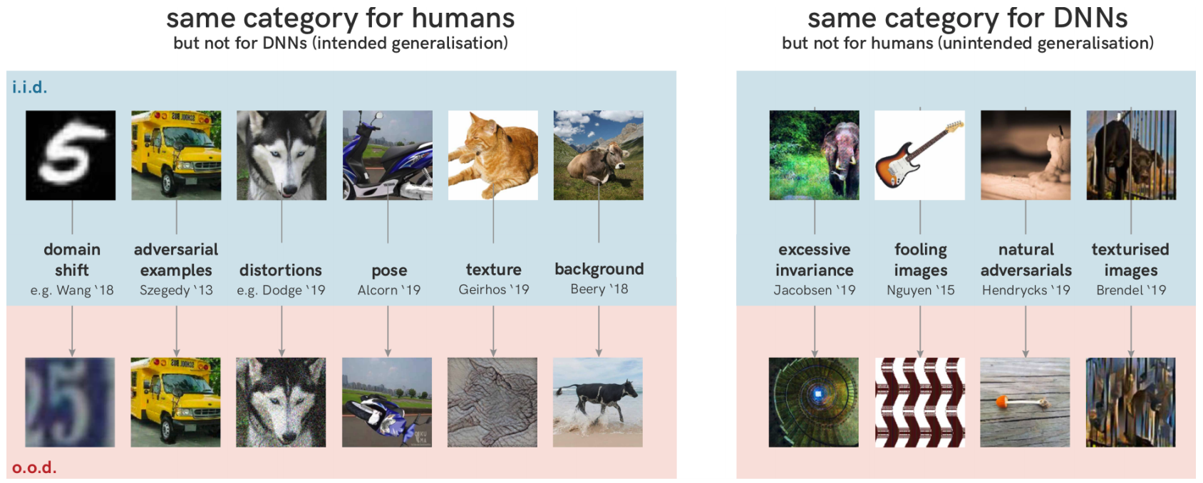
Figure 15: Examples of generalization failures. From Geirhos et al. (2020), Figure 3, p. 8, reprinted with permission, and unaltered. Original caption: “Both human and machine vision generalise, but they generalise very differently. Left: image pairs that belong to the same category for humans, but not for DNNs. Right: image pairs assigned to the same category by a variety of DNNs, but not by humans.” - The common ILSVRC benchmark involves classifying images from 1000 categories. But humans can plausibly classify objects from more (much more?) than 10,000 categories, including very particular categories like “that one mug” or “the chair from the living room.”[533]Jenkins et al. (2018) for example, found that “people know about 5000 faces on average” (p. 1) and Biederman (1987) estimates that people know 30,000 distinguishable object categories, though he treats this as “liberal” (e.g., on the high end). I have not attempted to evaluate his … Continue reading Indeed, it’s unclear to me, conceptually, how to draw the line between classifying an object (“house,” “dog,” “child”) and thinking/feeling/predicting (“house I’d like to live in,” “dog that I love,” “child in danger”).[534]Another example might be an image-classification task that involves classifying images into “funny” and “not funny” – a task hardly limited in difficulty by the number of basic objects humans can identify. See Karpathy (2012) for discussion of all of the complex understanding that goes … Continue reading That said, it’s possible that all of these categories draw on similar low-level visual features detected in early stages of processing.
- The resolution of the human visual system may be finer than the resolution of typical ImageNet images. The optic nerve has roughly 1 million retinal ganglion cells that carry input from the retina, and the retina as a whole has about 100 million photoreceptor cells.[535] Dr. Dario Amodei suggested this consideration. Sarpeshkar (2010) treats the retina as receiving 36Gb/s, and outputing 20 Mb/s (p. 749, he cites Koch et al. (2004)). A typical input to an image classifier is 224 × 224 × 3: ~150,000 input values (though some inputs are larger).[536] See here: “224×224×3, a typical size for an image classifier.” See here for some example input sizes.
That said, DNNs may also be superior to the human visual system in ways. For example, Geirhos et al. (2018) compared DNN and human performance at identifying objects presented for 200 ms, and found that DNNs outperformed humans by >5% classification accuracy on images from the training distribution (humans generally did better overall when the images were altered).[537]Geirhos et al. (2018): “Here we proposed a fair and psychophysically accurate way of comparing network and human performance on a number of object recognition tasks: measuring categorization accuracy for single-fixation, briefly presented (200 ms) and backward-masked images as a function of … Continue reading And human vision is subject to its own illusions, blind spots, shortcuts, etc.[538]From Open Philanthropy’s non-verbatim notes from a conversation with Dr. Kate Storrs: “On the other hand, a lot of our impression of the richness of human vision is illusory. For example, we don’t see crisply, or in color, in the periphery of our visual field. So perhaps biological vision … Continue reading And I certainly don’t know that many species of dog. Overall, though, the human advantages here seem more impressive to me.
Note, also, that the question here is not whether DNNs are processing visual information exactly like humans do. For example, in order to qualify as human-level, the models don’t need to make the same sorts of mistakes humans do. What matters is high-level task performance.
Making up some numbers
Suppose we forge ahead with a very loose functional method estimate, despite these uncertainties. What results?
An EfficientNet-B2, capable of a roughly human-level 95% top-five accuracy on ImageNet classification, takes 1e9 FLOPs for a forward pass – though note that if we assume sparse FLOPs (e.g., no costs for multiplying by or adding 0), as we did for the mechanistic method, this number would be lower;[539] This is a point suggested by Dr. Dario Amodei. The Cerebras whitepaper suggests that “50 to 98% of your multiplications are wasted” on non-sparse hardware (p. 5). and it might be possible to prune/compress the model further (though EfficientNet-B2 is already optimized to minimize FLOPs).[540]Ravi (2018): “For example, on ImageNet task, Learn2Compress achieves a model 22× smaller than Inception v3 baseline and 4× smaller than MobileNet v1 baseline with just 4.6-7% drop in accuracy. On CIFAR-10, jointly training multiple Learn2Compress models with shared parameters, takes only 10% … Continue reading
Humans can recognize ~ten images per second (though the actual process of assigning labels to ImageNet images takes much longer).[541]From Open Philanthropy’s non-verbatim notes from a conversation with Prof. Won Mok Shim: “There is a fair amount of consensus in the field that the human visual system can recognize about ten images per second (e.g., one image per 100 ms). However, this doesn’t mean that it takes 100 ms to … Continue reading If we ran EfficientNet-B2 ten times per second, this would require ~1e10 FLOP/s.
On one estimate from 1995, V1 in humans has about 3e8 neurons.[542] Carandini (2012): “Thanks to high neuronal density and large area, V1 contains a vast number of neurons. In humans, it contains about 140 million neurons per hemisphere (Wandell, 1995), i.e. about 40 V1 neurons per LGN neuron” (from the introduction). However, based on more recent estimates in chimpanzees, I think this estimate might be low, possibly by an order to magnitude (see endnote for explanation).[543]For example, one recent estimate by Miller et al. (2014), using better methods, finds 675 million neurons for chimpanzee V1 as a whole. Another – Collins et al. (2016) – finds 737 million neurons in just onechimpanzee V1 hemisphere, suggesting ~1.4 billion in V1 as a whole. The human cortex … Continue reading I’ll use 3e8-3e9 – e.g., ~0.3%-3% of the brain’s neurons.
On an initial search, I haven’t been able to find good sources for neuron count in the visual cortex as a whole, which includes areas V2-V5.[544] Though Collins et al. (2016) find ~400 million in one hemisphere on chimpanzee V2, suggesting 800 million for chimp V2 as a whole, and 1.6 billion for human V2, if we assume similar ratios in the cortex. I’ll use 1e9-1e10 neurons – e.g., ~1-10% of the brain’s neurons as a whole – but this is just a ballpark.[545]The high-end here is more than half of the neurons in the cortex as a whole (~16 billion neurons, according to Azevedo et al. (2016) (p. 536), which seems high to me, based on eyeballing pictures of the visual cortex. That said, neuron density in primate visual cortex appears to be unusually high … Continue reading
If we focused on percentage of volume, weight, energy consumption, and synapses, the relevant percentages might be larger (since the cortex accounts for a larger percentage of these than of the brain’s neurons).[546]See my discussion of the cerebellum in Section 2.4.2.3. Though note that neuron densities in V1 are especially high. See Collins et al. (2016): “the packing densities of neurons in V1 were 1.2, 2.1, 3.3, and 3.5 times greater than neuron densities in secondary visual cortex (V2) and … Continue reading
We can distill the other uncertainties from 3.2.1 and 3.2.2 into two numbers:
- The percentage of its information-processing capacity that the visual cortex devotes to tasks analogous to image classification, when it performs them.
- The factor increase in FLOP/s required to reach human-level performance on this task (if any), relative to the FLOP/s costs of an EfficientNet-B2 run 10 times per second.
Absent a specific chunk of the visual cortex devoted exclusively to this task, the percentage in (1) does not have an obvious physiological interpretation in terms of e.g. volume or number of neurons.[547] One could also ask questions like: “how many fewer neurons could this region have/how much less energy could it use, if evolution got to rebuild it from scratch, without needing to do task X, but still needing to do everything else it does?” But these are hard to answer. Still, something like percentage of spikes or of signaling-based energy consumption driven by performing the task might be a loose guide.[548]Drexler (2019) appears to have something like this in mind: “A key concept in the following will be “immediate neural activity” (INA), an informal measure of potentially task-applicable brain activity. As a measure of current neural activity potentially applicable to task performance, INA is … Continue reading
Of course, the resources that a brain uses in performing a task are not always indicative of the FLOP/s the task requires. Multiplying two 32-bit numbers in your head, for example, uses lots of spikes, energy, etc., but requires only one FLOP. And naively, it seems unlikely that the neural resources used in playing e.g. Tic-Tac-Toe, Checkers, Chess, and Go will be a simple function of the FLOP/s that have thus far been found necessary to match human-level performance. However, the brain was not optimized to multiply large numbers or play board games. Identifying visual objects (e.g. predators, food) seems like a better test of its computational potential.[549] My thanks to Dr. Eric Drexler for discussion.
Can we say anything about (1)? Obviously, it’s difficult. The variance in the activity in the visual cortex explained by DNN image classifiers might provide some quantitative anchor (this appears to be at least 7% in V1, and possibly much higher in other regions), but I haven’t explored this much.[550]Here’s one loose attempt to estimate (1). Following the data in Cadena et al. (2019), suppose that for half of the neurons in V1, ~28% of the variance is explained by the visual stimulus, and ~50% of that can be explained by networks trained on object recognition. To be conservative, let’s … Continue reading Still, to the extent (1) makes sense at all, it should be macroscopic enough to explain the results discussed at the beginning of this section (e.g., it should make interesting parallels between the feature detection in DNNs and the visual cortex noticeable using tools like fMRI and spike recordings), along with other modeling successes in visual neuroscience I haven’t explored.[551]See e.g. Open Philanthropy’s non-verbatim notes from a conversation with Dr. Kate Storrs: “In Dr. Storrs’ area of neuroscience, there can be a narrative to the effect that: “the early visual system is basically done. We understand the canonical computations: e.g., edge, orientation and … Continue reading I’ll use 1% of V1 as a low end,[552] Open Philanthropy’s technical advisor, Dr. Dario Amodei, suggests that V1 might be a helpful point of focus (ImageNet models plausibly cover functions in other parts of the visual cortex, but he suggests that basing estimates on V1 is conservative). and 10% of the visual cortex as a whole as a high end, with 1% of the visual cortex as a rough middle.
My biggest hesitation about these numbers comes from the conceptual ambiguities involved in estimating this type of parameter at all. Consider: “what fraction of a horse’s legs does a wheelbarrow automate?”[553] This is a variant on an analogy suggested by Nick Beckstead. It’s not clear that “of course it’s hard to say precisely, but surely at least a millionth, right?” is a sensible answer – and the problem isn’t that the true answer is a billionth instead. It seems possible that comparisons between DNNs and the visual cortex are similar.
We also need to scale up the size of the DNN in question by (2), to reflect the FLOPs costs of fully human-level image classification. What is (2)? I haven’t looked into it much, and I feel very uncertain. Some of the differences discussed in 3.2.2 – for example, differences in input size, or in number of categories (assuming we can settle on a meaningful estimate for the number of categories humans can recognize) – might be relatively easy to adjust for.[554] For example, FLOPs scaling for bigger inputs appears to be roughly linear: see e.g. here. Dr. Dario Amodei also suggested linear scaling for bigger inputs as a conservative adjustment. But others, such as the FLOPs required to run models that are only as vulnerable to adversarial examples as humans are, or that can generalize as well as humans can, might involve much more involved and difficult extrapolations.
I’m not going to explore these adjustments in detail here. Here are a few possible factors:
- 10x (150k input values vs. ~1 million retinal ganglion cells)
- 100x (~factor increase in EfficientNet-B2 FLOPs required to run a BiT-L model, which exhibits better, though still imperfect, generalization to real-world datasets like ObjectNet).[555]Kolesnikov et al. (2020): “All of our BiT models use a vanilla ResNet-v2 architecture [16], except that we replace all Batch Normalization [21] layers with Group Normalization [60] and use Weight Standardization [43] in all convolutional layers. See Section 4.3 for analysis. We train ResNet-152 … Continue reading
- 1000x (10x on top of a Bit-L model, for additional improvements. I basically just pulled this number out of thin air, and it’s by no means an upper bound).
Putting these estimates for (1) and (2) together:
| ESTIMATE TYPE | ASSUMED PERCENTAGE OF VISUAL CORTEX INFORMATION-PROCESSING CAPACITY USED FOR TASKS ANALOGOUS TO IMAGE CLASSIFICATION, WHEN PERFORMED | IMPLIED PERCENTAGE OF THE WHOLE BRAIN’S CAPACITY (BASED ON NEURON COUNT) | ASSUMED FACTOR INCREASE IN 10 HZ EFFICIENTNET-B2 FLOP/S (1E10) REQUIRED TO REACH FULLY HUMAN-LEVEL IMAGE CLASSIFICATION | WHOLE BRAIN FLOP/S ESTIMATE RESULTING FROM THESE ASSUMPTIONS |
|---|---|---|---|---|
| Low-end | 10% | 0.1%-1% | 10x | 1e13-1e14 |
| Middle | 1% | 0.01%-0.1% | 100x | 1e15-1e16 |
| High-end | 0.3% (1% of V1) | 0.003%-0.03% | 1000x | 3e16-3e17 |
Obviously, the numbers for (1) and (2) here are very made-up. The question of how high (2) could go, for example, seems very salient. And the conceptual ambiguities involved in comparing what the human visual system is doing when it classifies an image, vs. what a DNN is doing, caution against relying on what might appear to be conservative bounds.
What’s more, glancing at different models, image classification (that is, assigning labels to whole images) appears to require fewer FLOPs than other vision tasks in deep learning, such as object detection (that is, identifying and localizing multiple objects in an image). For example: an EfficientDet-D7, a close to state of the art object-detection model optimized for efficiency, uses 3e11 FLOPs per forward pass – 300x more than an EfficientNet-B2.[556] Tan et al. (2020): “In particular, with single-model and single test-time scale, our EfficientDet-D7 achieves state-of-the-art 53.7 AP with 52M parameters and 325B FLOPs, outperforming previous best detector [44] with 1.5 AP while being 4× smaller and using 13× fewer FLOPs” (p. 2). So using this sort of model as a baseline instead could add a few orders of magnitude. And such a choice would raise its own questions about what human-level performance on the relevant task looks like.
Overall, I hold functional method estimates based on current DNN vision models very lightly – even more lightly, for example, than the mechanistic method estimates above. Still, I don’t think them entirely uninformative. For example, it is at least interesting to me that you need to treat an EfficientNet-B2 as running on e.g. ~0.1% of the FLOPs of a model that would cover ~1% of V1, in order to get whole brain estimates substantially above 1e17 FLOP/s – the top end of the mechanistic method range I discussed above. This weakly suggests to me that such a range is not way too low.
Other functional method estimates
There are various other functional method estimates in the literature. Here are three:[557]Others not included in the chart include Kurzweil’s (2012) for a “pattern recognition”: “emulating one cycle in a single pattern recognizer in the biological brain’s neocortex would require about 3,000 calculations. Most simulations run at a fraction of this estimate. With the brain … Continue reading
| SOURCE | TASK | ARTIFICIAL SYSTEM | COSTS OF HUMAN-LEVEL PERFORMANCE | ESTIMATED PORTION OF BRAIN | RESULTING ESTIMATE FOR WHOLE BRAIN |
|---|---|---|---|---|---|
| Drexler (2019)[558]Drexler (2019): “Baidu’s Deep Speech 2 system can approach or exceed human accuracy in recognizing and transcribing spoken English and Mandarin, and would require approximately 1 GFLOP/s per real-time speech stream (Amodei et al. 2015). For this roughly human-level throughput, fPFLOP = 10−6 … Continue reading | Speech recognition | DeepSpeech2 | 1e9 FLOP/s | >0.1% | 1e12 FLOP/s |
| Drexler (2019)[559]Drexler (2019): “Google’s neural machine translation (NMT) systems have reportedly approached human quality (Wu et al. 2016). A multi-lingual version of the Google NMT model (which operates with the same resources) bridges language pairs through a seemingly language-independent representation … Continue reading | Translation | Google Neural Machine Translation | 1e11 FLOP/s (1 sentence per second) | 1% | 1e13 FLOP/s |
| Kurzweil (2005)[560]Kurzweil (2005): “Another estimate comes from the work of Lloyd Watts and his colleagues on creating functional simulations of regions of the human auditory system, which I discuss further in chapter 4. One of the functions of the software Watts has developed is a task called “stream … Continue reading | Sound localization | Work by Lloyd Watts | 1e11 calculations/s | 0.1% | 1e14 calculations/s |
I haven’t attempted to vet these estimates. And we can imagine others. Possibly instructive recent work includes:
- Kell et al. (2018), who suggest that ANNs trained to recognize sounds can predict neural activity in the cortex.[561]Kell et al. (2018): “…we optimized hierarchical neural networks for speech and music recognition. The best-performing network contained separate music and speech pathways following early shared processing, potentially replicating human cortical organization. The network performed both tasks as … Continue reading
- Banino et al. (2018) and Cueva and Wei (2018), who suggest that ANNs trained on navigation tasks develop grid-like representations, akin to grid cells in biological circuits.[562]Banino et al. (2018): “Grid cells are thought to provide a multi-scale periodic representation that functions as a metric for coding space7,8 and is critical for integrating self-motion (path integration)6,7,9 and planning direct trajectories to goals (vector-based navigation)7,10,11. Here we … Continue reading
- Merel et al. (2020), who develop a virtual rodent, which might allow productive comparison with the capabilities of a real rodent.[563]Merel et al. (2020): “In this work we develop a virtual rodent that learns to flexibly apply a broad motor repertoire, including righting, running, leaping and rearing, to solve multiple tasks in a simulated world. We analyze the artificial neural mechanisms underlying the virtual rodent’s … Continue reading
That said, I expect other functional method estimates to encounter difficulties analogous to those discussed in section 3.2: e.g., difficulties identifying (a) the percentage of the brain’s capacity devoted to a given task, (b) what human-level performance looks like, and (c) the FLOP/s sufficient to match this level.
The limit method
Let’s turn to a third method, which attempts to upper bound required FLOP/s by appealing to physical limits.
Some such bounds are too high to be helpful. Lloyd (2000), for example, calculates that a 1 kg, 1 liter laptop (the brain is roughly 1.5 kg and 1.5 liters) can perform a maximum of 5e50 operations per second, and store a maximum of 1e31 bits. Its memory, though, “looks like a thermonuclear explosion.”[564]Lloyd (2000): “The amount of information that can be stored by the ultimate laptop, ≈ 1031 bits, is much higher than the ≈ 1010 bits stored on current laptops. This is because conventional laptops use many degrees of freedom to store a bit where the ultimate laptop uses just one. There are … Continue reading For present purposes, such idealizations aren’t informative.
Other physical limits, though, might be more so. I’ll focus on “Landauer’s principle,” which specifies the minimum energy costs of erasing bits (more description below). Standard FLOPs (that is, the FLOPs performed by human-engineered computers) erase bits, which means that an idealized computer running on the brain’s energy budget (~20W) can only perform so many standard FLOP/s: specifically, ~7e21 (~1e21 if we assume 8-bit FLOPs, and ~1e19 if we assume current digital multiplier implementations).[565] See calculations in Section 4.2.
Does this upper bound the FLOP/s required to match the brain’s task-performance? In principle, no. The brain need not be performing operations that resemble standard FLOPs, and more generally, bit-erasures are not a universal currency of computational complexity.[566] My thanks to Prof. David Wallace for discussion. In theory, for example, factorizing a semiprime requires no bit-erasures, since the mapping from inputs to outputs is 1-1.[567] My thanks to Prof. David Wallace for suggesting this example. But we’d need many FLOPs to do it. Indeed, in principle, it appears possible to perform arbitrarily complicated computations with very few bit erasures, with manageable algorithmic overheads (though there is at least some ongoing controversy about this).[568]From Open Philanthropy’s non-verbatim notes from a conversation with Dr. Paul Christiano: “The algorithmic overhead involved in reversible computing (specifically, the overhead involved in un-computing what you have already computed) is not that bad. Most of the difficulty lies in designing … Continue reading
Absent a simple upper bound, then, the question is what we can say about the following quantity:
FLOP/s required to match the brain’s task performance ÷ bit-erasures/s in the brain
Various experts I spoke to about the limit method (though not all[569]From Open Philanthropy’s non-verbatim notes from a conversation with Dr. Michael Frank (p. 2): Dr. Frank thinks that it is possible that there are processes in the brain that are close to thermodynamically reversible, and that play a role in computation. We don’t know enough about the brain … Continue reading) thought it likely that this quantity is less than 1 – indeed, multiple orders of magnitude less.[570]From Open Philanthropy’s non-verbatim notes from a conversation with Prof. Jared Kaplan (p. 2): Mr. Carlsmith asked Prof. Kaplan’s opinion of the following type of upper bound on the compute required to replicate the brain’s task-performance. According to Landauer’s principle, the brain, … Continue reading They gave various arguments, which I’ll roughly group into (a) algorithmic arguments (Section 4.2.1), and (b) hardware arguments (Section 4.2.2). Of these, the hardware arguments seem to me stronger, but they also don’t seem to me to rely very directly on Landauer’s principle in particular.
Whether the bound in question emerges primarily from Landauer’s principle or not, though, I’m inclined to defer to the judgment of these experts overall.[571] This deference is not merely the result of tallying up the amount of expert support for different perspectives: it incorporates many more subjective factors involved in my evaluation of the overall evidence the expert opinions I was exposed to provides. And even if their arguments to do not treat the brain entirely as a black box, a number of the considerations these arguments appeal to seem to apply in scenarios where more specific assumptions employed by other methods are incorrect. This makes them an independent source of evidence.
Note, as well, that e.g. 1e21 FLOP/s isn’t too far from some of the numbers that have come up in previous sections. And some experts either take numbers in this range or higher seriously, or are agnostic about them.[572]From Open Philanthropy’s non-verbatim notes from a conversation with Prof. Konrad Kording: “Examination of neurons reveals that they are actually very non-linear, and the computations involved in plasticity probably include a large number of factors distributed across the cell. In this sense, … Continue reading In this sense, the bound in question, if sound, would provide an informative constraint.
Bit-erasures in the brain
Landauer’s principle
Landauer’s principle says that implementing a computation that erases information requires transferring energy to the environment – in particular, k × T × ln2 per bit erased, where k is Boltzmann’s constant, and T is the absolute temperature of the environment.[573]I’ve mostly relied on Frank (2018), Sagawa (2014), Wolpert (2019), and Wolpert (2019a) for my understanding of the principle, together (centrally) with discussion with experts. Feyman (1996), Chapter 5, also contains a fairly accessible introduction. See Landauer (1961) for the original … Continue reading
I’ll define a computation, here, as a mapping from input logical states to probability distributions over output logical states, where logical states are sets of physical microstates treated as equivalent for computational purposes;[574]Here I am following Frank (2018): “Let there be a countable (usually finite) set C = {ci} of distinct entities ci called computational states. Then a general definition of a (possibly stochastic) (computational) operation O is a function O : C → P(C), where P(C) denotes the set of probability … Continue reading and I’ll use “operation” to refer to a comparatively basic computation implemented as part of implementing another computation. Landauer’s principle emerges from the close relationship between changes in logical entropy (understood as the Shannon entropy of the probability distribution over logical states) and thermodynamic entropy (understood as the natural logarithm of the number of possible microstates, multiplied by Boltzmann’s constant).[575]Schroeder (2000): “Entropy is just the logarithm of the number of ways of arranging things in the system (times Boltzmann’s constant)” (p. 75). See also Wikipedia on Boltzmann’s principle. From Open Philanthropy’s non-verbatim notes from a conversation with Prof. Jared Kaplan: … Continue reading
In particular, if (given an initial probability distribution over inputs) a computation involves decreasing logical entropy (call a one bit decrease a “logical bit-erasure”),[576]I am using the term “logical bit-erasures” to quantify logical entropy drops of the kind to which Landauer’s principle, as I understand it, is relevant, even in a stochastic context. Discussions of Landauer’s principle sometimes assume a deterministic context, in which the relationship … Continue reading then implementing this computation repeatedly using a finite physical system (e.g., a computer) eventually requires increasing the thermodynamic entropy of the computer’s environment – otherwise, the total thermodynamic entropy of the computer and the environment in combination will decrease, in violation of the second law of thermodynamics.[577]My (non-expert) understanding is that one way to loosely and informally express the basic idea here (without attempting to actually justify it technically) is that because the computer and the environment areassumed to be independent (at least with respect to the types of correlations we will … Continue reading
Landauer’s principle quantifies the energy costs of this increase.[578]From Open Philanthropy’s non-verbatim notes from a conversation with Dr. Jess Riedel: “In certain rare environments, you can decrease entropy by paying costs in conserved quantities other than energy (for example, you can pay costs in angular momentum). But this is not relevant in the context … Continue reading These costs arise from the relationship between the energy and the thermodynamic entropy of a system: broadly, if a system’s energy increases, it can be in more microstates, and hence its entropy increases.[579]From Open Philanthropy’s non-verbatim notes from a conversation with Dr. Jess Riedel: “Landauer’s principle follows almost trivially from basic principles of thermodynamics. Indeed, it can be understood simply as a rewriting of the definition of temperature. At a fundamental level, … Continue reading Temperature, fundamentally, is defined by this exchange rate.[580]Schroeder (2000): “The temperature of a system is the reciprocal of the slope of its entropy vs. energy graph. The partial derivative is to be taken with the system’s volume and number of particles held fixed; more explicitly: 1/T = (dS/dUf)N,V (3.5). From now on I will take equation 3.5 to be … Continue reading
There has been some controversy over Landauer’s principle,[581]See Bennett (2003), section 2 (“Objections to Landauer’s principle”), for a description of the various objections, together with his replies (p. 502-508). Some aspects of the controversy, such as whether Landauer’s principle can exorcise Maxwell’s Demon without first assuming the second … Continue reading and some of the relevant physics has been worked out more rigorously since Landauer’s original paper.[582]Wolpert (2019a): “This early work [by Landauer and Bennett] was grounded in the tools of equilibrium statistical physics. However, computers are highly nonequilbrium systems. As a result, this early work was necessarily semiformal, and there were many questions it could not address. On the other … Continue reading But the basic thrust emerges from very fundamental physics, and my understanding is that it’s widely accepted by experts.[583]Prof. David Wallace indicated that most physicists accept Landauer’s principle. Though see Open Philanthropy’s non-verbatim notes from a conversation with Dr. Jess Riedel: “Landauer’s principle follows almost trivially from basic principles of thermodynamics… There is some dispute over … Continue reading A number of recent results also purport to have validated Landauer’s principle empirically.[584]See the review in Frank (2018): “In 2012, Berut et al. tested Landauer’s Principle in the context of a colloidal particle trapped in a modulated double-well potential, an experimental setup designed to mimic the conceptual picture that we reviewed in Fig. 12. Their experimental results showed … Continue reading
Overall bit-erasures
Let’s assume that Landauer’s principle caps the bit-erasures the brain can implement. What bit-erasure budget does this imply?
Most estimates I’ve seen of the brain’s energy budget vary between ~10-20W (Joules/second).[585]Aiello (1997): “On the basis of in vivo determinations, the mass-specific metabolic rate of the brain is approximately 11.2 W/kg (watts per kilogram). This is over 22 times the mass-specific metabolic rate of skeletal muscle (0.4 W/kg) (Aschoff et al. (1971)). A large brain would, therefore, be … Continue reading But not all of this energy goes to computation:
- Loose estimates suggest that 40% of energy use in the brain,[586]Engl and Attwell (2015): “Current theoretical estimates and experimental data assessing the contribution of each ‘housekeeping’ process to the brain’s total energy budget are inconclusive for many processes, varying widely in some cases. Further research is needed to fill these gaps, and … Continue reading and 25% in cortical gray matter,[587]See Howarth et al. (2012): “As panel A, but including non-signaling energy use, assumed to be 6.81 × 10²² ATP/s/m3, that is, 1/3 of the neuronal signaling energy, so that housekeeping tasks are assumed to account for 25% of the total energy use. On this basis, resting potentials use 15%, … Continue reading goes towards non-signaling tasks.[588]See Engl and Attwell (2015) for some description of these tasks: “Perhaps surprisingly, a significant fraction of brain energy use (25–50%) in previous energy budgets has been assigned to non-signalling (so-called ‘housekeeping’) tasks, which include protein and lipid synthesis, proton … Continue reading
- Some signaling energy is plausibly used for moving information from one place to another, rather than computing with it. Harris and Attwell (2012), for example, estimate that action potentials use 17% of the energy in grey matter (though much less in white matter).[589] See Figure 1.
That said, these don’t initially appear to be order-of-magnitude level adjustments. I’ll use 20W as a high end.
The brain operates at roughly 310 Kelvin, as does the body.[590]Wang et al. (2014): “On average, deep brain temperature is less than 1°C higher than body temperature in humans, unless cerebral injury is severe enough to significantly disrupt the brain-body temperature regulation (Soukup et al., 2002)” (p. 6). Thanks to Asya Bergal for this citation. See … Continue reading Even if the air surrounding the body is colder, Dr. Jess Riedel suggested that it’s the temperature of the skull and blood that’s relevant, as the brain has to push entropy into the environment via these conduits.[591]From Open Philanthropy’s non-verbatim notes from a conversation with Dr. Jess Riedel: “The temperature relevant to applying Landauer’s limit to the brain is essentially that of the skull and blood. Even if the temperature outside the body is at a lower temperature, the brain will have to … Continue reading
At 310 K, k × T × ln2 Joules results in a minimum energy emission of 3e-21 Joules per bit erasure.[592] See calculation here. With a 20W budget, this allows no more than 7e21 bit erasures per second in the brain overall.[593]See calculation here. Sandberg’s (2016) estimate is slightly higher: “20 W divided by 1.3 × 10⁻²¹ J (the Landauer limit at body temperature) suggests a limit of no more than 1.6 × 10²² irreversible operations per second” (p. 5). This is because his estimate of the Landauer limit at body … Continue reading This simple estimate passes over some complexities (see endnote), but I’ll use it as a first pass.[594]From Open Philanthropy’s non-verbatim notes from a conversation with Prof. David Wolpert: “In Prof. Wolpert’s view, it is a subtle and interesting question how to do this type of calculation correctly. A rigorous version would require a large research project. One complexity is that the … Continue reading
From bit-erasures to FLOP/s
Can we get from this to a bound on required FLOP/s?
If the brain were performing standard FLOPs, it would be easy. A standard FLOP takes two n-bit numbers, and produces another n-bit number. So absent active steps to save the inputs, you’ve erased at least n bits.[595]Jared Kaplan’s notes on Statistical Mechanics & Thermodynamics: “Say we add two numbers, eg 58 + 23 = 81. We started out with information representing both 58 and 23. Typically this would be stored as an integer, and for example a 16 bit integer has information, or entropy, 16 log 2. But at … Continue reading 7e21 bit-erasures/s, then, would imply a maximum of e.g. ~2e21 4-bit FLOP/s, 9e20 8-bit FLOP/s, and so forth, for a computer running on 20W at 310 Kelvin.
And the intermediate steps involved in transforming inputs into outputs erase bits as well. For example, Hänninen et al. (2011) suggest that on current digital multiplier implementations, the most efficient form of n-bit multiplication requires 8 × n2 bit-erasures – e.g., 128 for a 4-bit multiplication, and 512 for an 8-bit multiplication.[596] Hänninen et al. (2011) estimate the bit-erasures implicated by various proposed multiplier implementations. The array multiplier is the most efficient, at 8n2 for n-bit words (see Table II, p. 2372). 8 × 42 = 128; 83 = 512. This would suggest a maximum of ~5e19 4-bit digital multiplications, and ~1e19 8-bit multiplications (though analog implementations may be much more efficient).[597]Sarpeshkar (1998) discusses more efficient, analog implementations: “Items 1 through 3 show that analog computation can be far more efficient than digital computation because of analog computation’s repertoire of rich primitives. For example, addition of two parallel 8-bit numbers takes one … Continue reading
And FLOPs in actual digital computers appear to erase even more bits than this – ~1 bit-erasure per transistor switch involved in the operation.[598] See also Hänninen et al. (2011): “Present CMOS effectively performs an erasure every time a transistor switches states—generating hugely unnecessary levels of heat” (p. 2370). Sarpeshkar (1998) suggests 3000 transistors for an 8-bit digital multiply (though only 4-8 in for analog implementations);[599] Sarpeshkar (1998): “an 8-bit multiplication of two currents in analog computation takes 4 to 8 transistors, whereas a parallel 8-bit multiply in digital computation takes approximately 3000 transistors” (p. 1605). Asadi and Navi (2007) suggest >20,000 for a 32-bit multiply.[600] Asadi and Navi (2007): “Table 3: comparison between 32 × 32 bit multipliers … Transistor counts: 21579.00, 25258.00, 32369.00” (Table 3, p. 346).
Perhaps for some, comfortable assuming that the brain’s operations are relevantly like standard FLOPs, this is enough. But a robust upper bound should not assume this. The brain implements some causal structure that allows it to perform tasks, which can in principle be replicated using FLOP/s, but which itself could in principle take a wide variety of unfamiliar forms. Landauer’s principle tells us that this causal structure, represented as a set of (possibly stochastic) transitions between logical states, cannot involve erasing more than 7e21 bits/second.[601] Given the probability distribution over inputs to which the brain is in fact exposed, that is. It doesn’t tell us anything, directly, about the FLOP/s required to replicate the relevant transitions, and/or perform the relevant tasks.[602] My thanks to Prof. David Wallace for discussion.
Here’s an analogy. Suppose that you’re wondering how many bricks you need to build a bridge across the local river, and you know that a single brick always requires a pound of mortar. You learn that the “old bridge” across the river was built using no more than 100,000 pounds of mortar. If the old bridge is made of bricks, then you can infer that 100,000 bricks is enough. If the old bridge is made of steel, though, you can’t: even assuming that a brick can do anything y units of steel can do, y units of steel might require less (maybe much less) than a pound of mortar, so the old bridge could still be built with more than 100,000×y units of steel.
Obviously, the connection between FLOPs, bit-erasures, and the brain’s operations may be tighter than that between bricks, mortar, and steel. But conceptually, the point stands: unless we assume that the brain performs standard FLOPs, moving from bit-erasures to FLOPs requires further arguments. I’ll consider two types.
We might think that any algorithm useful for information-processing, whether implemented using standard FLOPs or no, will require erasing lots of logical bits.
In theory, this appears to be false (though there is at least some ongoing controversy, related to the bit-erasures implied by repeatedly reading/writing inputs and outputs).[603]From Open Philanthropy’s non-verbatim notes from a conversation with Dr. Jess Riedel: “There is a simple algorithm for converting a computation that uses logically irreversible operations into an equivalent computation that uses logically reversible operations. This allows you to avoid almost … Continue reading Any computation can be performed using logically reversible operations (that is, operations that allow you to reconstruct the input on the basis of the output), which do not erase bits.[604]Sagawa (2014): “A computational process C is logically reversible if and only if it is an injection. In other words, C is logically reversible if and only if, for any output logical state, there is a unique input logical state. Otherwise, C is logically irreversible” (p. 7 in the arxiv … Continue reading For example, in theory, you can make multiplication reversible just by saving one of the inputs.[605]Hänninen and Takala (2010): “the logical reversal of the addition requires the result word and n extra bits, which could be chosen simply to represent one of the input operands” (p. 224). And see also Jared Kaplan’s notes on Statistical Mechanics & Thermodynamics: “In principle we can … Continue reading And my understanding is that the algorithmic overheads involved in using logically reversible operations, instead of logically irreversible ones – e.g., additional memory to save intermediate results, additional processing time to “rewind” computations[606]Johnson (1999): “Efficient as such a system would be, there would still be drawbacks. In a complex calculation, the extra memory needed to save all the intermediary ”garbage bits” can grow wildly. As a compromise, Dr. Bennett devised a memory-saving method in which a computer would carry out … Continue reading – are fairly manageable, something like a small multiplicative factor in running time and circuit size.[607]From Open Philanthropy’s non-verbatim notes from a conversation with Dr. Jess Riedel: “For large computations, this conversion adds only a modest overhead in required time and memory. For example, the algorithm described in Charles Bennett’s 1989 paper ‘Time/Space Trade-Offs for Reversible … Continue reading
In practice, however, two experts I spoke with expected the brain’s information-processing to involve lots of logical bit-erasures. Reasons included:
- When humans write software to perform tasks, it erases lots of bits.[608] From Open Philanthropy’s non-verbatim notes from a conversation with Dr. Jess Riedel: “When humans write software to accomplish human objectives, they use a lot of irreversible steps (though there are some non-atomic reversible intermediate computations, like Fourier transforms)” (p. 4).
- Dr. Jess Riedel suggested that processing sensory data requires extracting answers to high-level questions (e.g., “should I dodge this flying rock to the left or the right?”) from very complex intermediate systems (e.g., trillions of photons hitting the eye), which involves throwing out a lot of information.[609]From Open Philanthropy’s non-verbatim notes from a conversation with Dr. Jess Riedel: “When the world has some simple feature (e.g., the position and velocity of a rock heading towards your head), this feature is encoded in very complicated intermediate systems (e.g., the trillions of photons … Continue reading
- Prof. Jared Kaplan noted that FLOPs erase bits, and in general, he expects order one bit-erasures per operation in computational systems. You generally don’t do a lot of complicated things with a single bit before erasing it (though there are some exceptions to this). His intuition about this was informed by his understanding of simple operations you can do with small amounts of information.[610]From Open Philanthropy’s non-verbatim notes from a conversation with Prof. Jared Kaplan: “FLOPs in actual computers erase bits, and Prof. Kaplan expects that you generally have order one bit-erasures per operation in computational systems. That is, you don’t do a lot of complicated things … Continue reading
If one imagines erasing lots of bits as the “default,” then you can also argue that the brain would need to be unrealistically energy-efficient (see next section) in order to justify any overheads incurred by transitioning to more reversible forms of computation.[611]From Open Philanthropy’s non-verbatim notes from a conversation with Dr. Jess Riedel: “if (as in current conventional computers) you’re dissipating thousands of kT per operation, it isn’t worth transitioning to logically reversible operations, because other forms of energy dissipation … Continue reading Dr. Paul Christiano noted, though, that if evolution had access to computational mechanisms capable of implementing useful, logically-reversible operations, brains may have evolved a reliance on them from the start.[612]From Open Philanthropy’s non-verbatim notes from a conversation with Dr. Paul Christiano: “Dr. Christiano does not think that logically irreversible operations are a more natural or default computational unit than reversible ones. And once we’re engaging with models of brain computation that … Continue reading
We can also look at models of neural computation to see what bit-erasures they imply. There is some risk, here, of rendering the limit method uninformative (e.g., if you’ve already decided how the brain computes, you can just estimate required FLOP/s directly).[613] My thanks to Prof. David Wallace for discussion. But it could still be helpful. For example:
- Some kinds of logical irreversibility may apply to large swaths of hypotheses about how the brain computes (e.g., hypotheses on which the membrane potential, which is routinely reset, carries task-relevant information).
- Some specific hypotheses (e.g., each neuron is equivalent to X-type of very large neural network) might imply bit-erasures incompatible with Landauer’s bound.
- If the brain is erasing lots of bits in one context, this might indicate that it does so elsewhere too, or everywhere.
Of course, it’s a further step from “the brain is probably erasing lots of logical bits” to “FLOP/s required to replicate the brain’s task-performance ÷ bit-erasures per second in the brain ≤1,” just as it’s a further step from “the old bridge was probably built using lots of mortar” to “bricks I’ll need ÷ pounds of mortar used for the old bridge ≤1.” One needs claims like:
- A minimal, computationally useful operation in the brain probably erases at least one logical bit, on average.
- One FLOP is probably enough to capture what matters about such an operation, on average.
Prof. Kaplan and Dr. Riedel both seemed to expect something like (1) and (2) to be true, and they seem fairly plausible to me as well. But the positive algorithmic arguments just listed don’t themselves seem to me obviously decisive.
Another class of arguments appeals to the energy dissipated by the brain’s computational mechanisms. After all, for required FLOPs per logical bit-erasure to be >1, it would need to be the case that required FLOPs per ~0.69kT of energy dissipation is >1 as well.
For example, in combination with (2) above, we might argue instead for:
1*. A minimal, computationally useful operation in the brain probably dissipates at least 0.69kT, on average
One possibly instructive comparison is with the field of reversible computing, which aspires to build computers that dissipate arbitrarily small amounts of energy per operation.[614] Michael Frank gives a summary of the development of the literature on reversible computing here (see paragraphs starting with “I’ll summarize a few of the major historical developments…”). This requires logically reversible algorithms (since otherwise, Landauer’s principle will set a minimum energy cost per operation), but it also requires extremely non-dissipative hardware – indeed, hardware that is close to thermodynamically reversible (e.g., its operation creates negligible amounts of overall thermodynamic entropy).
Useful, scalable hardware of this kind would need to be really fancy. As Dr. Michael Frank puts it, it would require “a level of device engineering that’s so precise and sophisticated that it will make today’s top-of-the-line device technologies seem as crude in comparison, to future eyes, as the practice of chiseling stone tablets looks to us today.”[615] See this 2014 interview with the Machine Intelligence Research Institute. According to Dr. Frank, the biggest current challenge centers on the trade-off between energy dissipation and processing speed.[616]From Open Philanthropy’s non-verbatim notes from a conversation with Dr. Michael Frank: “The biggest challenge is figuring out the fundamental physics involved in improving the trade-offs between energy dissipation and speed in reversible processes. We don’t know of any fundamental limits in … Continue reading Dr. Christiano also mentioned challenges imposed by an inability to expend energy in order to actively set relevant physical variables into particular states: the computation needs to work for whatever state different physical variables happen to end up in.[617]From Open Philanthropy’s non-verbatim notes from a conversation with Dr. Paul Christiano: “In irreversible computers, you do not need to keep track of and take into account what happens to each degree of freedom, because you are able to expend energy to reset the system to a state it needs to … Continue reading
For context, the energy dissipation per logical bit-erasure in current digital computers appears to be ~1e5-1e6 worse than Landauer’s limit, and progress is expected to asymptote between 1e3 and 1e5.[618]This is based primarily on eyeballing the chart presented at 4:17 in Michael Frank’s 2017 YouTube talk (Frank cites the International Roadmap of Semiconductors 2015, though I’m not sure where the specific information he’s pointing to comes from). According to Frank’s description of this … Continue reading A V100 GPU, at 1e14 FLOP/s and 300W, requires ~1e9 0.69kT per FLOP (assuming room temperature).[619] See calculation here. So in order to perform the logically-reversible equivalent of a FLOP for less than 0.69kT, you’d need a roughly billion-fold increase in energy efficiency.
Of course, biological systems have strong incentives to reduce energy costs.[620]See Aiello’s (1997) for some discussion. From Open Philanthropy’s non-verbatim notes from a conversation with Prof. David Wolpert: “Metabolic constraints are extremely important in evolutionary biology. But the field of evolutionary biology has not adequately incorporated discoveries about … Continue reading And some computational processes in biology are extremely efficient.[621]See e.g. Kempes et al. (2017): “Here we show that the computational efficiency of translation, defined as free energy expended per amino acid operation, outperforms the best supercomputers by several orders of magnitude, and is only about an order of magnitude worse than the Landauer bound” … Continue reading But relative to a standard of 0.69kT per operation, the brain’s mechanisms generally appear highly dissipative.[622]From Open Philanthropy’s non-verbatim notes from a conversation with Dr. Michael Frank: “In general, Dr. Frank does not see evidence that biology is attempting to do anything like what human engineers working on reversible computing are trying to do. Reversible computing is an extremely … Continue reading For example:
- Laughlin et al. (1998) suggest that synapses and cells use ~1e5-1e8kT per bit “observed” (though I don’t have a clear sense of what the relevant notion of observation implies).[623]See Laughlin et al. (1998): “Synapses and cells are using 105 to 108 times more energy than the thermodynamic minimum. Thermal noise sets a lower limit of k · T Joules for observing a bit of information (k, Boltzmann’s constant; T, absolute temperature, 290K) and the hydrolysis of one ATP … Continue reading
- A typical cortical spike dissipates around 1e10-1e11kT.[624]Lennie (2003) writes that “The aggregate cost of a spike is 2.4 × 10⁹ ATP molecules” (p. 493), and with Laughlin et al. (1998), who write that “the hydrolysis of one ATP molecule to ADP releases about 25 kT” (p. 39) (see also discussion here). 2.4e9 × 25 = 6e10. See also Bennett … Continue reading Prof. David Wolpert noted that this process involves very complicated physical machinery, which he expects to be very far from theoretical limits of efficiency, being used to propagate a single bit.[625]From Open Philanthropy’s non-verbatim notes from a conversation with Prof. David Wolpert: “Prof. Wolpert also expects that using Landauer’s principle to estimate the amount of computation performed by the brain will result in substantial overestimates. A single neuron uses very complicated … Continue reading
- Dr. Riedel mentioned that the nerves conveying a signal to kick your leg burn much more than 0.69kT per bit required to say how much to move the muscle.[626]From Open Philanthropy’s non-verbatim notes from a conversation with Dr. Jess Riedel: “Presumably, we think we basically understand cases where the brain is sending very simple signals, like the signal to kick your leg. We know that the nerves involved in conveying these signals are operating … Continue reading
- A single molecule of ATP (the brain’s main energy currency) releases ~25kT,[627]Laughlin et al. (1998) write that “the hydrolysis of one ATP molecule to ADP releases about 25 kT” (p. 39) (see also discussion here). Sarpeshkar (2014) also mentions “20 kT per molecular operation (1 ATP molecule hydrolysed)” (section 1). Swaminathan (2008) characterize ATP as … Continue reading and Dr. Christiano was very confident that the brain would need at least 10 ATPs to get computational mileage equivalent to a FLOP.[628]From Open Philanthropy’s non-verbatim notes from a conversation with Dr. Paul Christiano: “Dr. Christiano would be extremely surprised if the brain got more computational mileage out of a single ATP than human engineers can get out of a FLOP, and he would be very willing to bet that it takes … Continue reading At a rough maximum of ~2e20 ATPs per second,[629]Calculation here. This link also lists 1e-19 J per molecule, and 30-60 kJ per mole. Lennie (2003) estimates a “gross consumption of 3.4 × 10²¹ molecules of ATP per minute” in the cortex, and that “in the normal awake state, cortex accounts for 44% of whole brain energy consumption,” … Continue reading this would suggest <2e19 FLOP/s.
Of course, the relevant highly-non-dissipative information-processing could be hiding somewhere we can’t see, and/or occurring in a way we don’t understand. But various experts also mentioned more general features of the brain that make it poorly suited to this, including:
- The size of its components.[630]From Open Philanthropy’s non-verbatim notes from a conversation with Prof. Jared Kaplan: “In general, Prof. Kaplan thinks it unlikely that big, warm things are performing thermodynamically reversible computations” (p. 3). From Open Philanthropy’s non-verbatim notes from a conversation … Continue reading
- Its warm temperature.[631] From Open Philanthropy’s non-verbatim notes from a conversation with Prof. Jared Kaplan: “In general, Prof. Kaplan thinks it unlikely that big, warm things are performing thermodynamically reversible computations” (p. 3).
- The need to boost signals in order to contend with classical noise.[632]From Open Philanthropy’s non-verbatim notes from a conversation with Prof. Jared Kaplan: “If you’re in a regime where there is some signal to noise ratio, and you make your signal big to avoid noise, you can’t be doing something thermodynamically reversible: the noise is creating waste … Continue reading
- Its reliance on diffusion to propagate information.[633]From Open Philanthropy’s non-verbatim notes from a conversation with Prof. Jared Kaplan: “Processes that involve diffusion also cannot be thermodynamically reversible. Diffusion increases entropy. For example, if you take two substances and mix them together, you have increased the entropy of … Continue reading
- The extreme difficulty of building reversible computers in general.[634]From Open Philanthropy’s non-verbatim notes from a conversation with Prof. Jared Kaplan (p. 3):In general, it’s extremely difficult to build reversible computers. For example, all of the quantum computers we have are very rudimentary (quantum computers are a type of reversible computer), and … Continue reading
All of this seems to me like fairly strong evidence for something like 1*.
Note, though, that Landauer’s principle isn’t playing a very direct role here. We had intended to proceed from an estimate of the brain’s energy budget, to an upper bound on its logical bit-erasures (via Landauer’s principle), to an upper bound on the FLOP/s required to match its task performance. But hardware arguments skip the middle step, and just argue directly that you don’t need more than one FLOP per 0.69kT used by the brain. I think that this is probably true, but absent this middle step, 0.69kT doesn’t seem like a clearly privileged number to focus on.
Overall weight for the limit method
Overall, it seems very unlikely to me that more than ~7e21 FLOP/s is required to match the brain’s task-performance. This is centrally because various experts I spoke to seemed confident about claims in the vicinity of (1), (1*), and (2) above; partly because those claims seem plausible to me as well; and partly because other methods generally seem to point to lower numbers.[635] The FLOP/s costs of the models in Beniaguev et al. (2020), Maheswaranathan et al. (2019), and Batty et al. (2017) are the most salient exception.
Indeed, lower numbers (e.g., 1e21 – ~ the maximum 8-bit irreversible FLOP/s a computer running on 20W at 310 Kelvin could perform, and 1e20 – the maximum number of required FLOP/s, assuming at least one ATP per required FLOP) seem likely to me to be overkill as well.[636] I don’t give much weight to the energy costs of current digital multiplier implementations, given that analog implementations may be much more efficient (see Sarpeshkar (1998) (p. 1605)).
That said, this doesn’t seem like a case of a hard physical limit imposing a clean upper bound. Even equipped with an application of the relevant limit to the brain (various aspects of this still confuse me – see endnote), further argument is required.[637]A number of my confusions center on theoretical issues related to identifying the set of the computations that a physical system can be said to implement (see Piccinini (2017) for an introduction). For example, a simulation of a physical system at any level of detail is interpretable as a set of … Continue reading And indeed, the arguments that seem most persuasive to me (e.g., hardware arguments) don’t seem to rely very directly on the limit itself. Still, we should take whatever evidence we can get.
The communication method
Let’s briefly discuss a final method (the “communication method”), which attempts to use the communication bandwidth in the brain as evidence about its computational capacity. I haven’t explored this much, but I think it might well be worth exploring.
Communication bandwidth, here, refers to the speed with which a computational system can send different amounts of information different distances.[638]In the context of human hardware, I’ll use the term to cover both on-chip memory bandwidth and bandwidth between chips, since brain-equivalent systems can use multiple chips; in some contexts, like a TPU, we might also include very short-distance communication taking place between ALUs. … Continue reading This is distinct from the operations per second that a system can perform (computation), but it’s just as hard a constraint on what the system can do.
Estimating the communication bandwidth in the brain is a worthy project in its own right. But it also might help with computation estimates. This is partly because the marginal value of additional computation and communication are related (e.g., too little communication and your computational units sit idle; too few computational units and it becomes less useful to move information around).
Can we turn this into a FLOP/s estimate? The basic form of the argument would be roughly:
- The profile of communication bandwidth in the brain is X.
- If the profile of the communication bandwidth in the brain is X, then Y FLOP/s is probably enough to match its task performance.
I’ll discuss each premise in turn.
Communication in the brain
One approach to estimating communication in the brain would be to identify all of the mechanisms involved in it, together with the rates at which they can send different amounts of information different distances.
- Axons are clearly a central mechanism here, and one in which a sizeable portion of the brain’s energy and volume have been invested.[639]Howarth et al. (2012), Figure 1, estimate that maintaining resting potentials uses 15% of the total energy in the cortex (20% of signaling energy in the cortex), and action potentials use 16% (21% of signaling energy). Synaptic processes account for an additional 44% (see p. 1224). Schlaepfer et … Continue reading There is a large literature on estimating the information communicated by action potentials.[640] See Dayan and Abbott (2001), Chapter 4 (p. 123-150); Zador (1998); Tsubo et al. (2012), Fuhrmann et al. (2001), Mainen and Sejnowski (1995), van Steveninck et al. (1997).
- Dendrites also seem important, though generally at shorter distances (and at sufficiently short distances, distinctions between communication and computation may blur).[641]From Open Philanthropy’s non-verbatim notes from a conversation with Dr. Paul Christiano: “One can also distinguish between the bandwidth available at different distances. Axons vary in length, shorter-distance communication in neurons occurs via dendrites, and at sufficiently short distances, … Continue reading
- Other mechanisms (e.g. glia, neuromodulation, ephaptic effects, blood flow – I’m less sure about gap junctions) are plausibly low-bandwidth relative to axons and dendrites.[642]See discussion in Section 2.3. From Open Philanthropy’s non-verbatim notes from a conversation with Dr. Paul Christiano: “There are other communication mechanisms in the brain (e.g., glia, neuromodulation, ephaptic effects), but Dr. Christiano expects that these will be lower-bandwidth than … Continue reading If so, this would simplify the estimate. And the resources invested in axons and dendrites would make it seem somewhat strange if the brain has other, superior forms of communication available.[643] From Open Philanthropy’s non-verbatim notes from a conversation with Dr. Paul Christiano: “the brain invests a sizeable portion of its energy and volume into communication via axons, which would be a strange investment if it had some other, superior communication mechanism available” (p. 2).
Dr. Paul Christiano suggests a rough estimate of ~10 bits per spike for axon communication, and uses this to generate the bounds of ~1e9 bytes/s of long-distance communication across the brain, 1e11 bytes/s of short-distance communication (where each neuron could access ~1e7 nearby neurons), and larger amounts of very short-distance communication.[644]From Open Philanthropy’s non-verbatim notes from a conversation with Dr. Paul Christiano: “You can roughly estimate the bandwidth of axon communication by dividing the firing rate by the temporal resolution of spiking. Thus, for example, if the temporal precision is 1 ms, and neurons are … Continue reading
Another approach would be to draw analogies with metrics used to assess the communication capabilities of human computers. AI Impacts, for example, recommends the traversed edges per second (TEPS) metric, which measures the time required to perform a certain kind of search through a random graph.[645]AI Impacts: “Traversed edges per second (TEPS) is a metric that was recently developed to measure communication costs, which were seen as neglected in high performance computing.8 The TEPS benchmark measures the time required to perform a breadth-first search on a large random graph, … Continue reading They treat neurons as vertices on the graph, synapses as edges, and spikes through synapses as traversals of edges, yielding an overall estimate of ~2e13-6e14 TEPS (the same as their estimate of the number of spikes through synapses).[646]Their estimate makes a number of assumptions, including that (1) most relevant communication is between neurons (as opposed to e.g. internal to neurons); (2) that traversing an edge is relevantly similar to spiking; (3) that the distribution of edges traversed doesn’t make a material difference, … Continue reading
I haven’t investigated either of these estimates in detail. But they’re instructive examples.
From communication to FLOP/s
How do we move from a communication profile for the brain, to an estimate of the FLOP/s sufficient to match its task performance? There are a number of possibilities.
One simple argument runs as follows: if you have two computers comparable on one dimension important to performance (e.g., communication), but you can’t measure how they compare on some other dimension (e.g., computation), then other things equal, your median guess should be that they are comparable on this other dimension as well.[647]Here I describe a specific version of a general type of argument suggested by Dr. Paul Christiano. From Open Philanthropy’s non-verbatim notes from a conversation with Dr. Paul Christiano: “Dr. Christiano puts some weight on the following type of a priori argument: if you have two computers … Continue reading Here, the assumption would be that the known dimension reflects the overall skill of the engineer, which was presumably applied to the unknown dimension as well.[648]The argument appears in a different light if all you know is that e.g. both computers are green (though even there, it would seem strange to think that e.g. the one on the left is probably better than the one on the right, if you have no information to distinguish them). My thanks to Paul … Continue reading As an analogy: if all we know is that Bob’s cheesecake crusts are about as good as Maria’s, the best median guess is that they’re comparable cheesecake chefs, and hence that his cheesecake filling is about as good as hers as well.
Of course, we know much about brains and computers unrelated to how their communication compares. But those drawn to simple a priori arguments, perhaps this sort of approach can be useful.
Using Dr. Christiano’s estimates, discussed above, one can imagine comparing a V100 GPU to the brain as follows:[649]From Open Philanthropy’s non-verbatim notes from a conversation with Dr. Paul Christiano: “A V100 GPU has about 1e12 bytes/s of memory bandwidth on the chip (~10x the brain’s 1e11 bytes of short-distance communication, estimated above), and 3e11 bytes/s of off-chip bandwidth (~300x the … Continue reading
| METRIC | V100 | HUMAN BRAIN |
|---|---|---|
| Short-distance communication | 1e12 bytes/s of memory bandwidth | 1e11 bytes/s to nearby neurons? (not vetted)[650] From Open Philanthropy’s non-verbatim notes from a conversation with Dr. Paul Christiano (p. 2-3). |
| Long-distance communication | 3e11 bytes/s of off-chip bandwidth | 1e9 bytes/s across the brain? (not vetted)[651] From Open Philanthropy’s non-verbatim notes from a conversation with Dr. Paul Christiano (p. 2-3). |
| Computation | 1e14 FLOP/s | ? |
On these estimates, the V100’s communication is at least comparable to the brain’s (indeed, it’s superior by between 10 and 300x). Naively, then, perhaps its computation is comparable (indeed, superior) as well.[652]From Open Philanthropy’s non-verbatim notes from a conversation with Dr. Paul Christiano: “If we knew nothing else about the brain, then, this might suggest that the brain’s computational capacity will be less than, or at least comparable to, a V100’s computational capacity (~1e14 FLOP/s) … Continue reading This would suggest 1e14 FLOP/s or less for the brain.
That said, it seems like a full version of this argument would include other available modes of comparison as well (continuing the analogy above: if you also know that that Maria’s jelly cheesecake toppings are much worse than Bob’s, you should take this into account too). For example, if we assume that synapse weights are the central means of storing memory in the brain,[653]From Open Philanthropy’s non-verbatim notes from a conversation with Dr. Kate Storrs: “Dr. Storrs’ sense is that, in the parts of the field she engages with most closely (e.g., systems level modeling, visual/cognitive/perceptual modeling, human behavior), and maybe more broadly, a large … Continue reading we might get:
| METRIC | V100 | HUMAN BRAIN |
|---|---|---|
| Memory | 3e10 bytes on chip | 1e14-1e15 synapses,[654] See Section 2.1.1. each storing >5 bits?[655] Bartol et al. (2015) suggest a minimum of “4.7 bits of information at each synapse” (they don’t estimate a maximum). |
| Power consumption | 300W | 20W[656] See Section 4.1.2. |
So the overall comparison here becomes more complicated. V100 power consumption is >10x worse, and comparable memory, on this naive memory estimate for the brain, would require a cluster of ~3000-30,000 V100s, suggesting a corresponding increase to the FLOP/s attributed to the brain (memory access across the cluster would become more complex as well, and overall energy costs would increase).[657] Here I’m treating a synapse weight as ~1 byte.
A related approach involves attempting to identify a systematic relationship between communication and computation in human computers – a relationship that might reflect trade-offs and constraints applicable to the brain as well.[658]From Open Philanthropy’s non-verbatim notes from a conversation with Dr. Paul Christiano: “In designing brains, evolution had to make trade-offs in allocating resources (e.g., energy consumption, space) to additional communication mechanisms, vs. additional mechanisms used for computation. … Continue reading Thus, for example, AI Impacts examines the ratio of TEPS to FLOP/s in eight top supercomputers, and finds a fairly consistent ~500-600 FLOP/s per TEPS.[659]See here: “The [eight] supercomputers measured here consistently achieve around 1-2 GTEPS per scaled TFLOPS (see Figure 3). The median ratio is 1.9 GTEPS/TFLOPS, the mean is 1.7 GTEPS/TFLOP, and the variance 0.14 GTEPS/TFLOP.” However, AI Impacts notes that they only looked at data about the … Continue reading Scaling up from their TEPS estimate for the brain, they get ~1e16-3e17 FLOP/s.[660]See here: “Among a small number of computers we compared4, FLOPS and TEPS seem to vary proportionally, at a rate of around 1.7 GTEPS/TFLOP. We also estimate that the human brain performs around 0.18 – 6.4 × 10¹⁴ TEPS. Thus if the FLOPS:TEPS ratio in brains is similar to that in computers, … Continue reading
A more sophisticated version of this approach would involve specifying a production function governing the returns on investment in marginal communication vs. computation.[661]From Open Philanthropy’s non-verbatim notes from a conversation with Dr. Paul Christiano: “Dr. Christiano’s approach requires some sort of production function relating the returns from investment in communication to investment in compute. Dr. Christiano’s starting point would be something … Continue reading This function might allow evaluation of different hypothesized combinations of communication and computation in the brain. Thus, for example, the hypothesis that the brain performs the equivalent of 1e20 FLOP/s, but has the communication profile listed in the table above, might face the objection that it assigns apparently sub-optimal design choices to evolution: e.g., in such a world, the brain would have been better served re-allocating resources invested in computation (energy, volume, etc.) to communication instead.
And even if the brain were performing the equivalent of 1e20 FLOP/s (perhaps because it has access to some very efficient means of computing), such a production function might also indicate a lower FLOP/s budget sufficient, in combination with more communication than the brain can mobilize, to match the brain’s task performance overall (since there may be diminishing returns to more computation, given a fixed amount of communication).[662]From Open Philanthropy’s non-verbatim notes from a conversation with Dr. Paul Christiano: “Such a production function would also allow you to estimate what it would take to match the overall performance of the brain, even without matching its compute capacity. Thus, for example, it’s … Continue reading
These are all just initial gestures at possible approaches, and efforts in this vein face a number of issues and objections, including:
- Variation in optimal trade-offs between communication and computation across tasks.
- Changes over time to the ratio of communication to computation in human-engineered computers.[663]From Open Philanthropy’s non-verbatim notes from a conversation with Dr. Paul Christiano: “One complication here is that the communication to computation ratio in human computers has changed over time. For example, traditional CPUs had less computation per unit communication than the current … Continue reading
- Differences in the constraints and trade-offs faced by human designers and evolution.
I haven’t investigated the estimates above very much, so I don’t put much weight on them. But I think approaches in this vicinity may well be helpful.
Conclusion
I’ve discussed four different methods of generating FLOP/s budgets big enough to perform tasks as well as the human brain. Here’s a summary of the main estimates, along with the evidence/evaluation discussed:
| ESTIMATE | DESCRIPTION | ~FLOP/S | SUMMARY OF EVIDENCE/EVALUATION |
|---|---|---|---|
| Mechanistic method low | ~1 FLOP per spike through synapse; neuron models with costs ≤ Izhikevich spiking models run with 1 ms time-steps. | 1e13-1e15 | Simple model, and the default in the literature; some arguments suggest that models in this vein could be made adequate for task-performance without major increases in FLOP/s; these arguments are far from conclusive, but they seem plausible to me, and to some experts (others are more skeptical). |
| Mechanistic method high | ~100 FLOPs per spike through synapse; neuron models with costs greater than Izhikevich models run with 1 ms time-steps, but less than single-compartment Hodgkin-Huxley run with 0.1 ms timesteps. | 1e15-1e17 | It also seems plausible to me that FLOP/s budgets for a fairly brain-like task-functional model would need to push into this range in order to cover e.g. learning, synaptic conductances, and dendritic computation (learning seems like an especially salient candidate here). |
| Mechanistic method very high | Budgets suggested by more complex models – e.g., detailed biophysical models, large DNN neuron models, very FLOPs-intensive learning rules. | >1e17 | I don’t see much strong positive evidence that you need this much, even for fairly brain-like models, but it’s possible, and might be suggested by higher temporal resolutions, FLOP/s intensive DNN models of neuron behavior, estimates based on time-steps per variable, greater biophysical detail, larger FLOPs budgets for processes like dendritic computation/learning, and/or higher estimates of parameters like firing rate or synapse count. |
| Scaling up the DNN from Beniaguev et al. (2020) | Example of an estimate >1e17 FLOP/s. Uses the FLOP/s for a DNN-reduction of a detailed biophysical model of a cortical neuron, scaled up by 1e11 neurons. | 1e21 | I think that this is an interesting example of positive evidence for very high mechanistic method estimates, as Beniaguev et al. (2020) found it necessary to use a very large model in order to get a good fit. But I don’t give this result on its own a lot of weight, partly because their model focuses on predicting membrane potential and individual spikes very precisely, and smaller models may prove adequate on further investigation. |
| Mechanistic method very low | Models that don’t attempt to model every individual neuron/synapse. | <1e13 | It seems plausible to me that something in this range is enough, even for fairly brain-like models. Neurons display noise, redundancy, and low-dimensional behavior that suggest that modeling individual neurons/synapses might be overkill; mechanistic method estimates based on low-level components (e.g. transistors) substantially overestimate FLOP/s capacity in computers we actually understand; emulation imposes overheads; and the brain’s design reflects evolutionary constraints that could allow further simplification. |
| Functional method estimate based on Moravec’s retina estimate, scaled up to whole brain | Assumes 1e9 calculations per second for the retina (100 calculations per edge/motion detection per, 10 edge/motion detections per second per cell, 1e6 cells); scaled up by 1e3-1e6 (the range suggested by portion of mass, volume, neurons, synapses, and energy). | 1e12-1e15 (assuming 1 calculation ~= 1 FLOP) | The retina does a lot of things other than edge and motion detection (e.g., it anticipates motion, it can signal that a predicted stimulus is absent, it can adapt to different lighting conditions, it can suppress vision during saccades); and there are lots of differences between the retina and the brain as a whole. But the estimate, while incomplete in its coverage of retinal function, might be instructive regardless, as a ballpark for some central retinal operations (I haven’t vetted the numbers Moravec uses for edge/motion detection, but Prof. Barak Pearlmutter expected them to be accurate).[664]See Open Philanthropy’s non-verbatim notes from a conversation with Prof. Barak Pearlmutter: “Prof. Hans Moravec attempted to derive estimates of the computational capacity of the brain from examination of the retina. Prof. Pearlmutter thought that Moravec’s estimates for the computational … Continue reading |
| Functional method estimate based on DNN models of the retina, scaled up to the whole brain | Estimates of retina FLOP/s implied by the models in Batty et al. (2017) (1e14 FLOP/s) and Maheswaranathan et al. (2019) (1e13 FLOP/s), scaled up to the brain as a whole using the same 1e3-1e6 range above. | 1e16-1e20 | I think this is some weak evidence for numbers higher than 1e17, and the models themselves are still far from full replications of retinal computation. However, I’m very uncertain about what it looks like to scale these models up to the retinas as a whole. And it also seems plausible to me that these models use many more FLOP/s than required to do what the retina does. For example, their costs reflect implementation choices and model sizes that haven’t yet been shown necessary, and Moravec’s estimate (even if incomplete) is much lower. |
| Low end functional method estimate based on the visual cortex | Treats a 10 Hz EfficientNet-B2 image classifier, scaled up by 10x, as equivalent to 10% of the visual cortex’s information-processing capacity, then scales up to the whole brain based on portion of neurons (portion of synapses, volume, mass, and energy consumption might be larger, if the majority of these are in the cortex). | 1e13-1e14 | In general, I hold these estimates lightly, as I feel very uncertain about what the visual cortex is doing overall and how to compare it to DNN image classifiers, as well as about the scale-up in model size that will be required to reach image classification performance as generalizable across data sets and robust to adversarial examples as human performance is (the high-end correction for this used here – 1000x – is basically just pulled out of thin air, and could be too low). That said, I do think that, to the extent it makes sense at all to estimate the % of the visual cortex’s information-processing capacity mobilized in performing a task analogous to image classification, the number should be macroscopic enough to explain the interesting parallels between the feature detection in image classifiers and in the visual cortex (see Section 3.2 for discussion). 1% of V1 seems to me reasonably conservative in this regard, especially given that CNNs trained on image classification end up as state of the art predictors of neural activity in V1 (as well as elsewhere in the visual cortex). So I take these estimates as some weak evidence that the mechanistic method estimates I take most seriously (e.g., 1e13-1e17) aren’t way too low. |
| Middle-range functional method estimate based on visual cortex | Same as previous, but scales up 10 Hz EfficientNet-B2 by 100x, and treats it as equivalent to 1% of the visual cortex’s information-processing capacity. | 1e15-1e16 | |
| High end functional method estimate based on visual cortex | Same as previous, but scales up 10 Hz EfficientNet-B2 by 1000x instead, and treats it as equivalent to 1% of V1’s information-processing capacity. | 3e16-3e17 | |
| Limit method low end | Maximum 8-bit, irreversible FLOP/s that a computer running on 20W at body temperature can perform, assuming current digital multiplier implementations (~500 bit-erasures per 8-bit multiply). | 1e19 | I don’t think that a robust version of the limit method should assume that the brain’s operations are analogous to standard, irreversible FLOP/s (and especially not FLOP/s in digital computers, given that there may be more energy-efficient analog implementations available – see Sarpeshkar (1998)). But it does seem broadly plausible to me that a minimal, computationally useful operation in the brain erases at least one logical bit, and very plausible that it dissipates at least 0.69kT (indeed, my best guess would be that it dissipates much more than that, given that cortical spikes dissipate 1e10-1e11kT; a single ATP releases ~25kT; the brain is noisy, warm, and reliant on comparatively large components, etc.). And it seems plausible, as well, that a FLOP is enough to replicate the equivalent of a minimal, computationally useful operation in the brain. Various experts (though not all) also seemed quite confident about claims in this vicinity. So overall, I do think it very unlikely that required FLOP/s exceeds e.g. 1e21. However, I don’t think this is a case of a physical limit imposing a clean upper bound. Rather, it seems like one set of arguments amongst others. Indeed, the arguments that seem strongest to me (e.g., arguments that appeal to the energy dissipated by the brain’s mechanisms) don’t seem to rely directly on Landauer’s principle at all. |
| Limit method middle | Maximum 8-bit, irreversible FLOP/s that a computer running in 20W at body temperature can perform, assuming no intermediate bit-erasures (just a transformation from two n-bit inputs to one n-bit output). | 1e21 | |
| Limit method high | Maximum FLOP/s, assuming at least one logical bit-erasure, or at least 0.69kT dissipation, per required FLOP. |
7e21 | |
| ATPs | Maximum FLOP/s, assuming at least one ATP used per required FLOP. | 1e20 | |
| Communication method estimate based on comparison with V100 | Estimates brain communication capacity, compares it to a V100, and infers on the basis of the comparability/inferiority of the brain’s communication to a V100s communication, perhaps it’s computational capacity is comparable/inferior as well. | ≤1e14 | I haven’t vetted these estimates much and so don’t put much weight on them. The main general question is whether the relationship between communication and computation in human-engineered computers provides much evidence about what to expect that relationship to be in the brain. Initial objections to comparisons to a V100, even granting the communication estimates for the brain that it’s based on, might center on complications introduced by also including memory and energy consumption in the comparison. Initial objections to relying on TEPS-FLOP/s ratios might involve the possibility that there are meaningfully more relevant “edges” in the brain than synapses, and/or “vertices” than neurons. Still, I think that approaches in this broad vicinity may well prove helpful on further investigation. |
| Communication method estimate based on TEPS to FLOP/s extrapolation | Estimates brain TEPS via an analogy between spikes through synapses and traversals of an edge in a graph; then extrapolates to FLOP/s based on observed relationship between TEPS and FLOP/s in a small number of human-engineered computers. | 1e16-3e17 FLOP/s |
Here are the main numbers plotted together:
None of these numbers are direct estimates of the minimum possible FLOP/s budget. Rather, they are different attempts to use the brain – the only physical system we know of that performs these tasks, but far from the only possible such system – to generate some kind of adequately (but not arbitrarily) large budget. If a given method is successful, it shows that a given number of FLOP/s is enough, and hence, that the minimum is less than that. But it doesn’t, on its own, indicate how much less.
Can we do anything to estimate the minimum directly, perhaps by including some sort of adjustment to one or more of these numbers? Maybe, but it’s a can of worms that I don’t want to open here, as addressing the question of where we should expect the theoretical limits of algorithmic efficiency to lie relative to these numbers (or, put another way, how many FLOP/s we should expect superintelligent aliens to use, if they were charged with replicating human-level task-performance using FLOPs) seems like a further, difficult investigation (though Dr. Paul Christiano expected the brain to be performing at least some tasks in close to maximally efficient ways, using a substantial portion of its resources – see endnote).[665]From Open Philanthropy’s non-verbatim notes from a conversation with Dr. Paul Christiano: “If you include a sufficiently broad range of tasks that the human brain can perform, and require similarly useful task-performance across the full range of inputs to which the brain could be exposed, it … Continue reading
Overall, I think it more likely than not that 1e15 FLOP/s is enough to perform tasks as well as the human brain (given the right software, which may be very hard to create). And I think it unlikely (<10%) that more than 1e21 FLOP/s is required. That said, as emphasized above:
- The numbers above are just very loose, back-of-the-envelope estimates.
- I am not a neuroscientist, and there is no consensus on this topic in neuroscience (or elsewhere).
- Basically all of my best-guesses are based on a mix of (a) shallow investigation of messy, unsettled science, and (b) a limited, non-representative sampling of expert opinion.
More specific probabilities require answering questions about the theoretical limits of algorithmic efficiency – questions that I haven’t investigated and that I don’t want to overshadow the evidence actually surveyed in the report. In the appendix, I discuss a few narrower conceptions of the brain’s FLOP/s capacity, and offer a few more specific probabilities there, keyed to one particular type of brain model. My current best-guess median for the FLOP/s required to run that particular type of model is around 1015 (recall that none of these numbers are estimates of the FLOP/s uniquely “equivalent” to the brain).
As can be seen from the figure above, the FLOP/s capacities of current computers (e.g., a V100 at ~1e14 FLOP/s for ~$10,000, the Fugaku supercomputer at ~4e17 FLOP/s for ~$1 billion) cover the estimates I find most plausible.[666]See here for V100 prices (currently ~$8799); and here the $1 billion Fugaku pricetag: “The six-year budget for the system and related technology development totaled about $1 billion, compared with the $600 million price tags for the biggest planned U.S. systems.” Fugaku FLOP/s performance … Continue reading However:
- Task-performance requires resources other than FLOP/s (for example, memory and memory bandwidth).
- Performing tasks on a particular machine can introduce further overheads and complications.
- Most importantly, matching the human brain’s task-performance requires actually creating sufficiently capable and computationally efficient AI systems, and this could be extremely (even prohibitively) difficult in practice even with computers that could run such systems in theory. Indeed, as noted above, the FLOP/s required to run a system that does X can be available even while the resources (including data) required to train it remain substantially out of reach. And what sorts of task-performance will result from what sorts of training is itself a further, knotty question.[667] See my colleague Ajeya Cotra’s investigation focuses on these issues.
So even if my best-guesses are correct, this does not imply that we’ll see AI systems as capable as the human brain anytime soon.
Possible further investigations
Here are a few projects that others interested in this topic might pursue (this list also doubles as a catalogue of some of my central ongoing uncertainties).
Mechanistic method
- Investigate the literature on population-level modeling and/or neural manifolds, and evaluate what sorts of FLOP/s estimates it might imply.
- Investigate the best-understood neural circuits (for example, Prof. Eve Marder mentioned some circuits in leeches, C. elegans, flies, and electric fish), and what evidence they provide about the computational models adequate for task-performance.[668] From Open Philanthropy’s non-verbatim notes from a conversation with Prof. Eve Marder: “There are also some circuits in leeches, C. elegans, flies, and electric fish that are relatively well-characterized” (p. 4).
- Follow up on the work in Beniaguev et al. (2020), testing different hypotheses about the size of deep neural networks required to fit neuron behavior with different levels of accuracy.
- Investigate the computational requirements and biological plausibility of different proposed learning rules in the brain in more depth.
- Investigate more deeply different possible hypotheses about molecular-level intracellular signaling processes taking place in the brain, and the FLOP/s they might imply.
- Investigate the FLOP/s implications of non-binary forms of axon signaling in more detail.
Functional method
- Following up on work by e.g. Batty et al. (2017) and Maheswaranathan et al. (2019), try to gather more data about the minimal artificial neural network models adequate to predict retinal spike trains across trials at different degrees of accuracy (including higher degrees of accuracy than these models currently achieve).
- Create a version of Moravec’s retina estimate that covers a wider range of computations that the retina performs, but which still focuses on high-level tasks rather than spike trains.
- Investigate the literature on comparisons between the feature detection in DNNs and in the visual cortex, and try to generate better quantitative estimates of the overlap and the functional method FLOP/s it would imply.
- Based on existing image classification results, try to extrapolate to the model size required to achieve human-level robustness to adversarial examples and/or generalization across image classification data sets.
- Investigate various other types of possible functional methods (for example, estimates based on ML systems performing speech recognition).
Limit method
- Investigate and evaluate more fleshed-out versions of algorithmic arguments.
- Look for and evaluate examples in biology where the limit method might give the wrong answer: e.g., where a biological system is performing some sort of useful computation that would require more than a FLOP to replicate, but which dissipates less than 0.69kT.
Communication method
- Estimate the communication bandwidth available in the brain at different distances.
- Investigate the trade-offs and constraints governing the relationship between communication and computation in human-engineered computers across different tasks, and evaluate the extent to which these would generalize to the brain.
General
- Gather more standardized, representative data about expert opinion on this topic.
- Investigate what evidence work on brain-computer interfaces might provide.
- Investigate and evaluate different methods of estimating the memory and/or number of parameters in the brain – especially ones that go beyond just counting synapses. What would e.g., neural manifolds, different models of state retention in neurons, models of biological neurons as multi-layer neural networks, dynamical models of synapses, etc., imply about memory/parameters?
- (Ambitious) Simulate a simple organism like C. elegans at a level of detail adequate to replicate behavioral responses and internal circuit dynamics across a wide range of contexts, then see how much the simulation can be simplified.
Appendix: Concepts of brain FLOP/s
It is reasonably common for people to talk about the brain’s computation/task-performance in terms of metrics like FLOP/s. It is much less common for them to say what they mean.
When I first started this project, I thought that there might be some sort of clear and consensus way of understanding this kind of talk that I just hadn’t been exposed to. I now think this much less likely. Rather, I think that there are a variety of importantly different concepts in this vicinity, each implying different types of conceptual ambiguity, empirical uncertainty, and relevant evidence. These concepts are sufficiently inter-related that it can be easy to slip back and forth between them, or to treat them as equivalent. But if offering estimates, or making arguments about e.g. AI timelines using such estimates, it matters which you have in mind.
I’ll group these concepts into four categories:
- FLOP/s required for task-performance, with no further constraints.
- FLOP/s required for task-performance + brain-like-ness constraints (e.g., constraints on the similarity between the task-functional model and the brain’s internal dynamics).
- FLOP/s required for task-performance + findability constraints (e.g., constraints on what sorts of processes would be able to create/identify the task-functional model in question).
- Other analogies with human-engineered computers.
I find it useful, in thinking about these concepts, to keep the following questions in mind:
- Single answer: Does this concept identify a single, well-defined number of FLOP/s?
- Non-arbitrariness. Does it involve a highly arbitrary point of focus?
- One-FLOP-per-FLOP: To the extent that this concept purports to represent the brain’s FLOP/s capacity, does an analogous concept, applied to a human-engineered computer, identify the number of FLOP/s that computer actually performs? E.g., applied to a V100, does it pick out 1e14 FLOP/s?[669]This is a criterion suggested by Dr. Paul Christiano. From Open Philanthropy’s non-verbatim notes from a conversation with Dr. Paul Christiano: “In thinking about conceptual standards to use in generating estimates for the FLOP/s necessary to run a task-functional model of a computational … Continue reading
- Relationship to the literature: To what extent do estimates offered in the literature on this topic (mechanistic method, functional method, etc.) bear on the FLOP/s this concept refers to?
- Relevance to AI timelines: How relevant is this number of FLOP/s to when we should expect humans to develop AI systems that match human-level performance?
This appendix briefly discusses some of the pros and cons of these concepts in light of such questions, and it offers some probabilities keyed to one in particular.
No constraints
This report has focused on the evidence the brain provides about the FLOP/s sufficient for task-performance, with no further constraints on the models/algorithms employed in performing the tasks. I chose this point of focus centrally because:
- Its breadth makes room for a wide variety of brain-related sources of evidence to be relevant.
- It avoids the disadvantages and controversies implied by further constraints (see below).
- It makes the discussion in the report more likely to be helpful to people with different assumptions and reasons for interest in the topic.
However, it has two main disadvantages:
- As noted in the report, evidence that X FLOP/s is sufficient is only indirect evidence about the minimum FLOP/s required; and the overall probability that X is sufficient depends, not just on evidence from the brain/current AI systems, but on further questions about where the theoretical limits of algorithmic efficiency are likely to lie. That said, as noted earlier, Dr. Paul Christiano expected there to be at least some tasks such (a) the brain’s methods of performing them are close to maximally efficient, and (b) these methods use most of the brain’s resources.[670]From Open Philanthropy’s non-verbatim notes from a conversation with Dr. Paul Christiano: “If you include a sufficiently broad range of tasks that the human brain can perform, and require similarly useful task-performance across the full range of inputs to which the brain could be exposed, it … Continue reading I haven’t investigated this, but if true, it would reduce the force of this disadvantage.
- The relevance of in principle FLOP/s requirements to AI timelines is fairly indirect. If you know that Y type of task-performance is impossible without X FLOP/s, then you know that you won’t see Y until X FLOP/s are available. But once X FLOP/s are available (as I think they probably are), the question of when you’ll see Y is still wide open. You know that superintelligent aliens could do it in theory, if forced to use only the FLOP/s your computers make available. But on its own, this gives you very little indication of when humans will do it in practice.
In light of these disadvantages, let’s consider a few narrower points of focus.
Brain-like-ness
One option is to require that models/algorithms employed in matching the brain’s task-performance exhibit some kind of resemblance to its internal dynamics as well. Call such requirements “brain-like-ness constraints.”
Such constraints restrict the set of task-functional models under consideration, and hence, to some extent, the relevance of questions about the theoretical limits of algorithmic efficiency. And they may suggest a certain type of “findability,” without building it into the definition of the models/algorithms under consideration. The brain, after all, is the product of evolution – a search and selection process whose power may be amenable to informative comparison with what we should expect the human research community to achieve.
But brain-likeness constraints also have disadvantages. Notably:
- From the perspective of AI timelines, it doesn’t matter whether the AI systems in question are brain-like.
- Functional method estimates are based on human-engineered systems that aren’t designed to meet any particular brain-like-ness constraints.
- It’s difficult to define brain-like-ness constraints in a manner that picks out a single, privileged number of FLOP/s, without making seemingly-arbitrary choices about the type of brain-like-ness in question and/or losing the One-FLOP-per-FLOP criterion above.
This last problem seems especially salient to me. Here are some examples where it comes up.
Brain simulations
Consider the question: what’s the minimum number of FLOP/s sufficient to simulate the brain? At a minimum, it depends on what you want the simulation to do (e.g., serve as a model for drug development? teach us how the brain works? perform a given type of task?). But even if we focus on replicating task-performance, there still isn’t a single answer, because we have not specified the level of brain-like-ness required to count as a simulation of the brain, assuming task-performance stays fixed.[671]From Open Philanthropy’s non-verbatim notes from a conversation with Prof. Rosa Cao: “Prof. Cao does not believe that there is a privileged description of the computations that the brain is performing. We can imagine many different possible computational models of the brain, which will … Continue reading Simulating individual molecules is presumably not required. Is replicating the division of work between hemispheres, but doing everything within the hemispheres in a maximally efficient but completely non-brain-like-way, sufficient?[672]From Open Philanthropy’s non-verbatim notes from a conversation with Dr. Paul Christiano: “In the case of the brain, for example, a high-level description might be something like ‘it divides the work between these two hemispheres in the following way.’ Thus, to meet the relevant standard, … Continue reading If so, we bring back many of the questions about the theoretical limits of algorithmic efficiency we were aiming to avoid. If not, where’s the line in between? We haven’t said.
“Reasonably brain-like” models
A similar problem arises if we employ a vaguer standard – requiring, for example, that the algorithm in question be “reasonably brain-like.” What counts? Are birds reasonably plane-like? Are the units of a DNN reasonably neuron-like? Some vagueness is inevitable, but this is, perhaps, too much.
Just picking a constraint
One way to avoid this would be to just pick a precisely-specified type of brain-likeness to require. For example, we might require that the simulation feature neuron-like units (defined with suitable precision), a brain-like connectome, communication via binary spikes, brain-like average firing rates, but not e.g. individual ion channels, protein dynamics, membrane potential fluctuations, etc. But why these and not others? Absent a principled answer, the choice seems arbitrary.
The brain’s algorithm
Perhaps we might appeal to the FLOP/s required to reimplement what I will call “the brain’s algorithm.” The idea, here, would be to assume that there is a single, privileged description of how the brain performs the tasks that it performs – a description that allows us to pick out a single, privileged number of FLOP/s required to perform those tasks in that way.
We can imagine appealing, here, to influential work by David Marr, who distinguished between three different levels of understanding applicable to an information-processing system:
- The computational level: the overall task that the system in question is trying to solve, together with the reason it is trying to solve this task.
- The algorithmic level: how the task-relevant inputs and outputs are represented in the system, together with the intermediate steps of the input-output transformation.
- The implementation level: how these representations and this algorithm are physically implemented.[673] See Marr (1982) (p. 25).
The report focused on level 1. But suppose we ask, instead: how many FLOP/s are required to replicate level 2? Again, the same problem arises: which departures from brain-like-ness are compatible with reimplementing the brain’s algorithm, and which are not (assuming high-level task performance remains unaffected regardless)? I have yet to hear a criterion that seems to me an adequate answer.[674]From Open Philanthropy’s non-verbatim notes from a conversation with Prof. Chris Eliasmith: “There is no privileged model of the brain which can claim to be the model of how the brain performs tasks. You can’t answer someone’s question about how the brain works without knowing exactly what … Continue reading
Note that this problem arises even if we assume clean separations between implementation and algorithmic levels in the brain – a substantive assumption, and one that may be more applicable in the context of human-engineered computers than biological systems.[675] See Bell (1999), Hanson (2011), and Lee (2011) for some discussion. For even in human-engineered computers, there are multiple algorithmic levels. Consider someone playing Donkey Kong on an MOS 6502. How many FLOP/s do you need to reimplement the “algorithmic level” of the MOS 6502, or to play Donkey Kong “the way the MOS 6502 does it”? I don’t think there’s a single answer. Do we need to emulate individual transistors, or are logic gates enough? Can we implement the adders, or the ALU, or the high-level architecture, in a different way? A full description of how the system performs the task involves all these levels of abstraction simultaneously. Given a description of an algorithm (e.g., a set of states and rules for transitioning between them), we can talk about the operations required to implement it.[676] E.g., we can talk about how many FLOP/s it takes to run an EfficientNet-B2 at 10 Hz, given a description of the model. But given an actual physical system operating on multiple levels of abstraction, it’s much less clear what talk about the algorithm it’s implementing refers to.[677] See Piccinini (2017) for discussion of related issues.
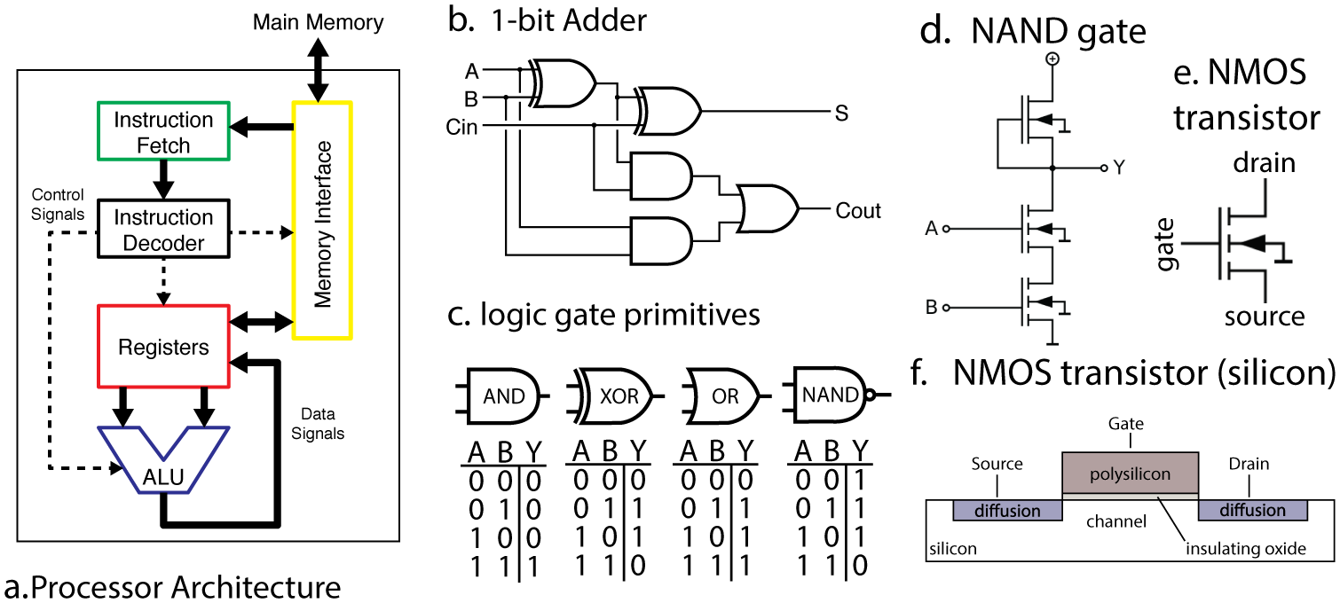
The lowest algorithmic level
Perhaps we could focus on the lowest algorithmic level, assuming this is well-defined (or, put another way, on replicating all the algorithmic levels, assuming that the lowest structures all the rest)? One problem with this is that even if we knew that a given type of brain simulation – for example, a connectome-like network of Izhikevich spiking neurons – could be made task-functional, we wouldn’t yet know whether it captured the level in question. Are ion channels above or below the lowest algorithmic level? To many brain modelers, these questions don’t matter: if you can leave something out without affecting the behavior you care about, all the better. But focusing on the lowest-possible algorithmic level brings to the fore abstract questions about where this level lies. And it’s not clear, at least to me, how to answer them.[678] For an example of the types of debates in this vein that do not seem to me particularly relevant or productive in this context, see here.
Another problem with focusing on the lowest algorithmic level is, to the extent that we want a FLOP/s estimate that would be to the brain what 1e14 FLOP/s is to a V100, we’ll do poorly on the One-FLOP-per-FLOP criterion above: e.g., if we assume that the lowest algorithmic level in a V100 is at the level of transistors, we’ll end up budgeting many more FLOP/s for a transistor-level simulation than the 1e14 FLOP/s the V100 actually performs.[679]From Open Philanthropy’s non-verbatim notes from a conversation with Dr. Paul Christiano: “Attempting to use some standard like “the description of the system you would give if you really understood how the system worked” might well result in over-estimates, since it would plausibly result … Continue reading
The highest algorithmic level
What about the highest algorithmic level? As with the lowest algorithmic level, it’s unclear where this highest level lies, and very high-level descriptions of the brain’s dynamics (analogous, e.g., to the “processor architecture” portion of the diagram above) may leave a lot of room for intuitively non-brain-like forms of efficiency (recall the “simulation” of the brain’s hemispheres discussed above). And it’s not clear that this standard passes the “one-FLOP-per-FLOP” test either: if a V100 performing some task is inefficient at some lower level of algorithmic description, then the maximally efficient way of performing that task in a manner that satisfies some higher level of description may use fewer FLOP/s than the V100 performs.
Nothing that doesn’t map to the brain
Nick Beckstead suggests a brain-like-ness constraint on which the algorithm used to match the brain’s task performance must be such that (a) all of its algorithmic states map onto brain states, and (b) the transitions between these algorithmic states mirror the transitions between the corresponding brain states.[680]This definition is based on the definition of when one computational method represents another offered by Knuth (1997), p. 467, problem 9. See also Sandberg and Bostrom (2008): “A strict definition of simulation might be that a system S consists of a state x(t) evolving by a particular dynamics … Continue reading Such a constraint rules out replicating the division of work between hemispheres, but doing everything else in a maximally efficient way, because the maximally efficient way will presumably involve algorithmic states that don’t map onto brain states.
This constraint requires specifying the necessary accuracy of the mapping from algorithmic states to brain states (though note that defining task-performance at all requires something like this).[681]See e.g. Sandberg and Bostrom (2008), who note that the brain is not strictly simulable on their definition, due to chaotic dynamics, but that “there exists a significant amount of noise in the brain that does not prevent meaningful brain states from evolving despite the indeterminacy of their … Continue reading I also worry that whether a given algorithm satisfies this constraint or not will end up depending on which operations are treated as basic (and hence immune from the requirement that the state-transitions involved in implementing them map onto the brain’s).[682]E.g., whether a given method of transitioning between states in a way that doesn’t map to the brain is OK or not will depend on whether this is construed as part of the “algorithm” or part of its “implementation.” But implementation itself takes place at many levels of abstraction, which … Continue reading And it’s not clear to me that this definition will capture One-FLOP-per-FLOP, since it seems to require a very high degree of emulation accuracy. That said, I think something in this vicinity might turn out to work.
More generally, though, brain-like-ness seems only indirectly relevant to what we ultimately care about, which is task-performance itself. Can findability constraints do better?
Findability
Findability constraints restrict attention to the FLOP/s required to run task-functional systems that could be identified or created via a specific type of process. Examples include task-functional systems that:
- humans will in fact create in the future (or, perhaps, the first such systems);
- humans would/could create, given access to a specific set of resources and/or data;
- would/could be identified via a specific type of training procedure – for example, a procedure akin to those used in machine learning today;
- could/would be found via a specified type of evolution-like search process, akin to the one that “found” the biological brain;
- could be created by an engineer “as good as evolution” at engineering.[683]See this post by AI impacts for a framework somewhat reminiscent of this conception, which plots indifference curves for different combinations of hardware and software sophistication. The post treats the brain as the point that combines “human-level hardware” and “evolution level software … Continue reading
The central benefit of all such constraints is that they are keyed directly to what it takes to actually create a task-functional system, rather than what systems could exist in principle. This makes them more informative for the purposes of thinking about when such systems might in fact be created by humans.
But it’s also a disadvantage, as estimates involving findability constraints require answering many additional, knotty questions about what types of systems are what kinds of findable (e.g., what sorts of research programs or training methods could result in what sorts of task performance; what types of resources and data these programs/methods would require; what would in fact result from various types of counterfactual “evolution-like” search processes, etc.).
Findability constraints related to evolution-like search processes/engineering efforts (e.g., (d) and (e) above) are also difficult to define precisely, and they are quite alien to mainstream neuroscientific discourse. This makes them difficult to solicit expert opinion about, and harder to evaluate using evidence of the type surveyed in the report.
My favorite of these constraints is probably the FLOP/s that will be used by the first human-built systems to perform these tasks, since this is the most directly relevant to AI timelines. I see functional method estimates as especially relevant here, and mechanistic/limit method estimates as less so.
Other computer analogies
There are a few other options as well, which appeal to various other analogies with human-engineered computers.
Operations per second
For example, we can imagine asking: how many operations per second does the brain perform? One problem here is that “operations” does not have a generic meaning. An operation is just an input-output relationship, implemented as part of a larger computation, and treated as basic for the purpose of a certain kind of analysis.[684]See discussion Schneider and Gersting (2018) (p. 96-100): “To measure time efficiency, we identify the fundamental unit (or units) of work of an algorithm and count how many times the work unit is executed” (p. 96). From Open Philanthropy’s non-verbatim notes from a conversation with Dr. … Continue reading The brain implements many different such relationships at different levels of abstraction: for example, it implements many more “ion-channel opening/closing” operations per second than it does “spikes through synapses” operations.[685] See e.g. Thagard (2002), who chooses to count proteins instead of neurons. Estimates that focus on the latter, then, need to say why they do so. You can’t just pick a thing to count, and count it.
More importantly, our ultimate interest is in systems that run on FLOP/s, that perform tasks at human-levels. To be relevant to this, then, we also need to know how many FLOP/s are sufficient to replicate one of the operations in question; and we need some reason to think that, so replicated, the resulting FLOP/s budget overall would be enough for task-performance. This amounts to something closely akin to the mechanistic method, and the same questions about the required degree of brain-like-ness apply.
FLOP/s it performs
What if we just asked directly: how many FLOP/s does the brain perform? Again, we need to know what is meant.
- One possibility is that we have in mind one of the other questions above: e.g., how many FLOP/s do you need to perform some set of tasks that the brain performs, perhaps with some kind of implicit brain-like-ness constraint. This raises the problems discussed in 7.1 and 7.2 above.
- Another possibility is that we are asking more literally: how many times per second does the brain’s biophysics implement e.g. an addition, subtraction, multiplication, or division operation of a given level of precision? In some places, we may be able to identify such implementation – for example, if synaptic transmission implements an addition operation via the postsynaptic membrane potential. In other places, though, the task-relevant dynamics in the brain may not map directly to basic arithmetic; rather, they may be more complicated, and require multiple FLOPs to capture. If we include these FLOPs (as we should, if we want the question to be relevant to the hardware requirements for advanced AI systems), we’re back to something closely akin to the mechanistic method, and to the same questions about brain-like-ness.
Usefulness limits
I’ll consider one final option, which seems to me (a) promising and (b) somewhat difficult to think about.
Suppose you were confronted with a computer performing various tasks, programmed by a programmer of unclear skill, using operations quite dissimilar from FLOP/s. You want some way of quantifying this computer’s computational capacity in FLOP/s. How would you do it?
As discussed above, using the minimum FLOP/s sufficient to perform any of the tasks the computer is currently programmed to perform seems dicey: this depends on where the theoretical limits of algorithmic efficiency lie, relative to algorithms the computer is running. But suppose we ask, instead, about the minimum FLOP/s sufficient to perform any useful task that the computer could in principle be programmed to perform, given arbitrary programming skill. An arbitrarily skillful programmer, after all, would presumably employ maximally efficient algorithms to use this computer to its fullest capacity.
Applied to a computer actually performing FLOP/s, this approach does well on the “One-FLOP-per-FLOP” criterion. That is, even an arbitrarily skillful programmer still cannot wring more FLOP/s out of a V100 than the computer actually performs, assuming this programmer is restricted to the computational mechanisms intended by the system’s designers. So the minimum FLOP/s sufficient to do any of the tasks that this programmer could use a V100 to perform would presumably be 1e14.
And it also fits well with what we’re intuitively doing when we ask about a system’s computational capacity: that is, we’re asking how useful this system can be for computational tasks. For instance, if a task requires 1e17 FLOP/s, can I do it with this machine? This approach gives the answers you would get if the machine actually performed FLOP/s itself.
Can we apply this approach to the brain? The main conceptual challenge, I think, is defining what sorts of interventions would count as “programming” the brain.[686]If we construe the type of task-performance at stake in the “no constraints” option above as including any task the brain can perform in the sense at stake here, then the two collapse into each other. However, my sense is that when people talk about matching human-level task-performance, they … Continue reading
- One option would be a restriction to external stimulation like e.g. talking, reading, etc. The tasks in question would be the set of tasks that any human could in principle be trained to perform, given arbitrary training time/arbitrarily skilled trainers. This would be limited by the brain’s existing methods of learning.
- Another option would be to allow direct intervention on biophysical variables in the brain. Here, the main problem would be putting limits on which variables can be intervened on, and by how much. Intuitively, we want to disallow completely remoulding the brain into a fundamentally different device, or “use” of mechanisms and variables that the brain does not currently “use” to store or process information. I think it possible that this sort of restriction can be formulated with reasonable precision, but I haven’t tried.
One might also object that this approach will focus attention on tasks that are overall much more difficult than the ones that we generally have in mind when we’re thinking about human-level task performance.[687] My thanks to Ajeya Cotra for discussion. I think that this is very likely true, but this seems quite compatible with using it as a concept of the brain’s FLOP/s capacity, as it seems fine (indeed, inuitive) if this concept indicates the limitations on the brain’s task performance imposed by hardware constraints alone, as opposed to other ways the system is sub-optimal.
Summing up
Here is a summary of the various concepts I’ve discussed:
| CONCEPT | ADVANTAGES | DISADVANTAGES |
|---|---|---|
| Minimum FLOP/s sufficient to match the brain’s task-performance | Simple; broad; focuses directly on task-performance. | Existing brains and AI systems provide only indirect evidence about the theoretical limits of algorithmic efficiency; questionably relevant to the FLOP/s we should expect human engineers to actually use. |
Minimum FLOP/s sufficient to run a task-functional model that meets some brain-like-ness constraint, such as being a:
|
Restricted space of models makes theoretical limits of algorithmic efficiency somewhat less relevant, and neuroscientific evidence more directly relevant; connection to evolution may indicate a type of findability (without needing to include such findability in the definition). | Non-arbitrary brain-like-ness constraints are difficult to define with precision adequate to pick out a single number of FLOP/s; the systems we ultimately care about don’t need to be any particular degree of brain-like; functional method estimates are not based on systems designed to be brain-like; analogous standards, applied to a human-engineered computer, struggle to identify the FLOP/s that computer actually performs; the connection between evolutionary find-ability and specific computational models of the brain is often unclear. |
Minimum FLOP/s sufficient to run a task-functional model that meets some findability constraint, such as being:
|
More directly relevant to the FLOP/s costs of models that we might expect humans to create, as opposed to ones that could exist in principle. “First model humans will in fact create” seems especially relevant (and functional method estimates may provide some purchase on it). | Implicating of difficult further questions about which models are what kinds of findable; findability constraints based on evolutionary hypotheticals/evolution-level engineers are also difficult to define precisely, and they are fairly alien from mainstream neuroscientific discourse – a fact which makes them difficult to solicit expert opinion about and/or evaluate using evidence of the type surveyed in the report. |
Other computer analogies:
|
Variable. Focusing on the tasks that the brain can be “programmed” to perform does fairly well on One-FLOP-per-FLOP, and it fits well with what we might want a notion of “FLOP/s capacity” to do, while also side-stepping questions about the degree of algorithmic inefficiency in the brain. | In order to retain relevance to task-functional systems running on FLOP/s, “operations per second in the brain” and “FLOP/s the brain performs” seem to me to collapse back into something like the mechanistic method, and to correspondingly difficult questions about the theoretical limits of algorithmic efficiency, and/or brain-like-ness. Focusing on the tasks that the brain can be programmed to perform requires defining what interventions count as “programming” as opposed to reshaping – e.g., distinguishing between hardware and software, which is hard in the brain. |
All these options have pros and cons. I don’t find any of them particularly satisfying, or obviously privileged as a way of thinking about the FLOP/s “equivalent” to the human brain. I’ve tried, in the body of the report, to use a broad framing; to avoid getting too bogged down in conceptual issues; and to survey evidence relevant to many narrower points of focus.
That said, it may be useful to offer some specific (though loose) probabilities for at least one of these. The point of focus I feel most familiar with is the FLOP/s required to run a task-functional model that satisfies a certain type of (somewhat arbitrary and ill-specified) brain-like-ness constraint, so I’ll offer some probabilities for that, keyed to the different mechanistic method ranges discussed above.
Best-guess probabilities for the minimum FLOP/s sufficient to run a task-functional model that satisfies the following conditions:
- It includes units and connections between units corresponding to each neuron and synapse in the human brain (these units can have further internal structure, and the model can include other things as well).[688] Strictly, they would need to correspond to the neurons and synapses in a particular human brain; but as I noted in Section 1.5, at the level of precision relevant to this report, I’m treating normal adult human brains as equivalent.
- The functional role of these units and connections in task-performance is roughly similar to the functional role of the corresponding neurons and synapses in the brain.[689] This is meant to exclude the possibility of using some other part of the model to do what is intuitively “all of the work,” but in some hyper-efficient manner.
Caveats:
- These are rough subjective probabilities offered about unsettled science. Hold them lightly.[690]In particular, despite the amount of evidence discussed in the report, I don’t think of these probabilities as particularly “robust.” Even in the final stages of this project, they’ve continued to vary somewhat as I’ve been exposed to new evidence, and as different considerations have … Continue reading
- (2) is admittedly imprecise. My hope is that these numbers can be a helpful supplement to the more specific evidence surveyed in the report, but those who think the question ill-posed are free to ignore.[691] The estimate can be seen as keyed to a concept that combines “just pick a degree of brain-like-ness” with “reasonably brain-like.” It has the disadvantages of both – namely, arbitrariness and vagueness.
- This is not an estimate of the “FLOP/s equivalent to the brain.” It’s an estimate of “the FLOP/s required to run a specific type of model of the brain.” See Sections 7.1–7.4 on why I think the concept of “the FLOP/s equivalent to the brain” is underspecified.
- I also think it very plausible that modeling every neuron/synapse is in some sense overkill (see Section 2.4.2) above), even in the context of various types of brain-like-ness constraints; and even more so without them.
- I assume access to “sparse FLOP/s,” as discussed inSection 2.1.1.2.2.
| FLOP/S RANGE | BEST-GUESS PROBABILITY | CENTRAL CONSIDERATIONS I HAVE IN MIND |
|---|---|---|
| <1e13 | ~15% | This is less than the estimate I’ve used for the spikes through synapses per second in the brain, so this range requires either that (a) this estimate is too high, or (b) satisfying the conditions above requires less than 1 FLOP per spike through synapse. (a) seems possible, as these parameters seem fairly unknown and I wouldn’t be that surprised if e.g. the average firing rate was <0.1 Hz, especially given the estimates in Lennie (2003). And (b) seems quite possible as well: a single FLOP might cover multiple spikes (for example, if what matters is a firing rate encoded in multiple spikes), and in general, it might well be possible to simplify what matters about the interactions between neurons in ways that aren’t salient to me (though note that simplifications that summarize groups of neurons are ruled out by the definition of the models in question).
This sort of range also requires <100 FLOP/s per neuron for firing decisions, which, assuming at least 1 FLOP per firing decision, means you have to be computing firing decisions less than 100 times per second. My naive guess would’ve been that you need to do it more frequently, if a neuron is operating on e.g. 1 ms timescales, but I don’t have a great sense of the constraints here, and Sarpeshkar (2010) and Dr. Paul Christiano both seemed to think it possible to compute firing decisions less than once per timestep (see Section 2.1.2.5). And finally, this sort of range requires that the FLOP/s required to capture the contributions of all the other processes described in the mechanistic method section (e.g., dendritic computation, learning, alternative signaling mechanisms, etc.) are <1 FLOP per spike through synapse and <100 FLOP/s per neuron. Learning seems to me like the strongest contender for requiring more than this, but maybe it’s in the noise due to slower timescales, and/or only a small factor (e.g., 2× for something akin to gradient descent methods) on top of a very low-end baseline. So overall, it doesn’t seem like this range is ruled out, even assuming that we’re modeling individual neurons and synapses. But it requires that the FLOPs costs of everything be on the low side. And my very vague impression that many experts (even those sympathetic to the adequacy of comparatively simple models) would think this range too low. That said, it also covers possible levels of simplification that current theories/models do not countenance. And it seems generally reasonable, in contexts with this level of uncertainty, to keep error bars (in both directions) wide. |
| 1e13-1e15 | ~30% | This is the range that emerges from the most common type of methodology in the literature, which budgets one operation per spike through synapse, and seems to assume that (i) operations like firing decisions, that scale with the number of neurons (~1e11) rather than number of synapses (~1e14-1e15), are in the noise, and (ii) so is everything else (including learning, alternative signaling mechanisms, and so on).
As I discuss in Section 2.1.2.5, I think that assumption (i) is less solid if we budget FLOPs at synapses based on spike rates rather than timesteps, since the FLOPs costs of processes in a neuron could scale with timesteps per neuron per second, and timesteps are plausibly a few orders of magnitude more frequent than spikes, on average. Still, this range covers all neuron models with FLOP/s costs less than an Izhikevich spiking neuron model run with 1 ms timesteps (~1e15 FLOP/s for 1e11 neurons) – a set that includes many models in the integrate-and-fire family (run at similar temporal resolutions). So it still seems like a decent default budget for fairly simple models of neuron/synapse dynamics. Dendritic computation and learning seem like prominent processes missing from such a basic model, so this range requires that these don’t push us beyond 1e15 FLOP/s. If we would end up on the low end of this range (or below) absent those processes, this would leave at least one or two orders of magnitude for them to add, which seems like a reasonable amount of cushion to me, given the considerations surveyed in Sections 2.1.2.2 and 2.2. That said, my best guess would be that we need at least a few FLOPs per spike through synapse to cover short-term synaptic plasticity, so there would need to be less than ~3e14 spikes through synapses per second to leave room for this. And most basic type of integrate-and-fire neuron model already puts us at ~5e14 FLOP/s (assuming 1 ms timesteps), so this doesn’t leave much room for increases from dendritic computation.[692] See Izhikevich (2004) (p. 1066); and the chart in Section 2.1.2.3. Overall, this range represents a simple default model that seems fairly plausible to me, despite not budgeting explicitly for these other complexities; and various experts appear to find this type of simple default persuasive.[693] See endnotes in Section 2.1.2.4 for examples. |
| 1e15-1e17 | ~30%. | This range is similar to the last, but with an extra factor of 100x budgeted to cover various possible complexities that came up in my research. Specifically, assuming the number of spikes through synapses falls in the range I’ve used (1e13-1e15), it covers 100-10,000 FLOPs per spike through synapse (this would cover Sarpeshkar’s (2010) 50 FLOPs per spike through synapse for synaptic filtering and learning; along with various models of learning discussed in Section 2.2.2) as well as 1e4-1e6 FLOP/s per neuron (this would cover, on the top end, single-compartment Hodgkin-Huxley models run with 0.1 ms timesteps – a level of modeling detail/complexity that I expect many computational neuroscientists to consider unnecessary).
Overall, this range seems very plausibly adequate to me, and various experts I engaged with seemed to agree.[694] See endnotes in Section 2.1.2.4. I’m much less confident that it’s required, but as mentioned above, my best guess is that you need at least a few FLOPs per spike through synapse to cover short-term synaptic plasticity, and plausibly more for more complex forms of learning; and it seems plausible to me that ultimately, FLOPs budgets for firing decisions (including dendritic computation) are somewhere between Izhikevich spiking neurons and Hodgkin-Huxley models. But as discussed above, lower ranges seem plausible as well. |
| 1e17-1e21 | ~20% | As I noted in the report, I don’t see a lot of strong positive evidence that budgets this high are required. The most salient considerations for me are (a) the large FLOP/s costs of various DNN models of neuron behavior discussed in the report, which could indicate types complexity that lower budgets do not countenance, and (b) if you budget at least one FLOP per timestep per synapse (as opposed to per spike through synapse), along with <1 ms timesteps, and>1e14 synapses, then you get above 1e17 FLOP/s, and it seems possible that sufficiently important and unsimplifiable changes are taking place at synapses this frequently (for example, changes involved in learning). Some experts also seem to treat “time-steps per second per variable” as a default method of generating FLOP/s estimates (and there may be many variables per synapse – see e.g. Benna and Fusi (2016)).
Beyond this, the other central pushes in this direction I feel involve (a) the general costliness of low-level modeling of biological and chemical processes; (b) the possibility that learning and dendritic computation introduce more complexity than 1e17 FLOP/s budgets for; (c) the fact that this range covers four orders of magnitude; (d) the possibility of some other type of unknown error or mistake, not currently on my radar, that pushes required FLOP/s into this range, and (e) an expectation that a decent number of experts would give estimates in this range as well. |
| >1e21 | ~5% | Numbers this high start to push past the upper bounds discussed in the limit method section. These bounds don’t seem airtight to me, but I feel reasonably persuaded by the hardware arguments discussed in Section 4.2.2 (e.g., I expect the brain to be dissipating at least a few kT per FLOP required to meet the conditions above, and to use at least 1 ATP, of which it has a maximum of ~1e20/s available). I also don’t see a lot of positive reason to go this high (though the DNN models I mentioned are one exception to this); other methods generally point to lower numbers; and some experts I spoke to were very confident that numbers in this range are substantial overkill. That said, I also put macroscopic probability on the possibility that these experts and arguments (possibly together with the broader paradigms they assume) are misguided in some way; that the conditions above, rightly understood, somehow end up requiring very large FLOP/s budgets (though this last one feels more like uncertainty about the concepts at stake in the question than uncertainty about the answer); and/or that the task-relevant causal structure in the brain is just intrinsically very difficult to replicate using FLOP/s (possibly because it draws on analog physical primitives, continuous/very fine-grained temporal dynamics, and/or complex biochemical interactions that are cheap for the brain, but very expensive to capture with FLOP/s). And in general, long tails seem appropriate in contexts with this level of uncertainty. |
Sources
| DOCUMENT | SOURCE |
|---|---|
| Aaronson (2011) | Source |
| Abraham and Philpot (2009) | Source |
| Achard and De Schutter (2006) | Source |
| Adam (2019) | Source |
| Adams (2013) | Source |
| Agarwal et al. (2017) | Source |
| AI Impacts, “Brain performance in FLOPS” | Source |
| AI Impacts, “Brain performance in TEPS” | Source |
| AI Impacts, “Glial Signaling” | Source |
| AI Impacts, “Neuron firing rates in humans” | Source |
| AI Impacts, “Scale of the Human Brain” | Source |
| AI Impacts, “The cost of TEPS” | Source |
| AI Impacts, “How AI timelines are estimated” | Source |
| Aiello (1997) | Source |
| Aiello and Wheeler (1995) | Source |
| Ajay and Bhalla (2006) | Source |
| Alger (2002) | Source |
| Amodei and Hernandez (2018) | Source |
| Amodei et al. (2016) | Source |
| Ananthanarayanan et al. (2009) | Source |
| Anastassiou and Koch (2015) | Source |
| Anastassiou et al. (2011) | Source |
| Andrade-Moraes et al. (2013) | Source |
| Angel et al. (2012) | Source |
| Antolík et al. (2016) | Source |
| Araque and Navarrete (2010) | Source |
| Araque et al. (2000) | Source |
| Araque et al. (2001) | Source |
| Arizona Power Authority, “History of Hoover” | Source |
| Arkhipov et al. (2018) | Source |
| Asadi and Navi (2007) | Source |
| Aschoff et al. (1971) | Source |
| Ashida et al. (2007) | Source |
| Astrup et al. (1981a) | Source |
| Attwell and Laughlin (2001) | Source |
| Azevedo et al. (2009) | Source |
| Backyard Brains, “Experiment: Comparing Speeds of Two Nerve Fiber Sizes” | Source |
| Balasubramanian and Berry (2002) | Source |
| Balasubramanian et al. (2001) | Source |
| Baldwin and Eroglu (2017) | Source |
| Banino et al. (2018) | Source |
| Barbu et al. (2019) | Source |
| Barth and Poulet (2012) | Source |
| Bartheld et al. (2016) | Source |
| Bartol et al. (2015) | Source |
| Bartol Jr et al. (2015) | Source |
| Bartunov et al. (2018) | Source |
| Bashivan et al. (2019) | Source |
| Batty et al. (2017) | Source |
| Bell (1999) | Source |
| Bengio et al. (2015) | Source |
| Beniaguev et al. (2019) | Source |
| Beniaguev et al. (2020) | Source |
| Benna and Fusi (2016) | Source |
| Bennett (1973) | Source |
| Bennett (1981) | Source |
| Bennett (1989) | Source |
| Bennett (2003) | Source |
| Bennett and Zukin (2004) | Source |
| Bennett et al. (1991) | Source |
| Bernardinell et al. (2004) | Source |
| Berry et al. (1999) | Source |
| Bezzi et al. (2004) | Source |
| Bhalla (2004) | Source |
| Bhalla (2014) | Source |
| Bi and Poo (2001) | Source |
| Bialowas et al. (2015) | Source |
| Biederman (1987) | Source |
| Bileh et al. (2020) | Source |
| Bindocci et al. (2017) | Source |
| Bischofberger et al. (2002) | Source |
| Blanding (2017) | Source |
| Blinkow and Glezer (1968) | Source |
| Bliss and Lømo (1973) | Source |
| Bollmann et al. (2000) | Source |
| Bomash et al. (2013) | Source |
| Bostrom (1998) | Source |
| Bouhours et al. (2011) | Source |
| Bower and Beeman (1995) | Source |
| Brain-Score | Source |
| Brain-Score, “Leaderboard” | Source |
| Brains in Silicon, “Publications” | Source |
| Braitenberg and Schüz (1998) | Source |
| Branco, Clark, and Häusser (2010) | Source |
| Brette (2015) | Source |
| Brette and Gerstner (2005) | Source |
| Brody and Yue (2000) | Source |
| Brown et al. (2020) | Source |
| Brownlee (2019a) | Source |
| Brownlee (2019b) | Source |
| Bruzzone et al. (1996) | Source |
| Bub (2002) | Source |
| Bucurenciu et al. (2008) | Source |
| Bullock et al. (1990) | Source |
| Bullock et al. (1994) | Source |
| Bullock et al. (2005) | Source |
| Burgoyne and Morgan (2003) | Source |
| Burke (2000) | Source |
| Burkitt (2006) | Source |
| Burr et al. (1994) | Source |
| Burrows (1996) | Source |
| Bush et al. (2015) | Source |
| Bushong et al. (2002) | Source |
| Bussler (2020) | Source |
| Büssow (1980) | Source |
| Butt et al. (2004) | Source |
| Button et al. (2013) | Source |
| Buzaki and Mizuseki (2014) | Source |
| Cadena et al. (2017) | Source |
| Cadena et al. (2019) | Source |
| Cantero et al. (2018) | Source |
| Carandini (2012) | Source |
| Carandini et al. (2005) | Source |
| Cariani (2011) | Source |
| Carp (2012) | Source |
| Carr and Boudreau (1993b) | Source |
| Carr and Konishi (1990) | Source |
| Castet and Masson (2000) | Source |
| Cell Biology By The Numbers, “How much energy is released in ATP hydrolysis?” | Source |
| Cerebras, “Cerebras Wafer Scale Engine: An Introduction” | Source |
| Chaigneau et al. (2003) | Source |
| Chang (2019) | Source |
| Cheng et al. (2018) | Source |
| Cheramy (1981) | Source |
| Chiang et al. (2019) | Source |
| Chong et al. (2016) | Source |
| Christie and Jahr (2009) | Source |
| Christie et al. (2011) | Source |
| Citri and Malenka (2008) | Source |
| Clark (2020) | Source |
| Clopath (2012) | Source |
| Cochran et al. (1984) | Source |
| Collel and Fauquet (2015) | Source |
| Collins et al. (2016) | Source |
| Compute Canada, “Technical Glossary” | Source |
| Cooke and Bear (2014) | Source |
| Cooke et al. (2015) | Source |
| Crick (1984) | Source |
| Crick (1989) | Source |
| Critch (2016) | Source |
| Cudmore and Desai (2008) | Source |
| Cueva and Wei (2018) | Source |
| Dalrymple (2011) | Source |
| Daniel et al. (2013) | Source |
| Dayan and Abbott (2001) | Source |
| De Castro (2013) | Source |
| de Faria, Jr. et al. (2019) | Source |
| Deans et al. (2007) | Source |
| Debanne et al. (2013) | Source |
| Deli et al. (2017) | Source |
| Deneve et al. (2001) | Source |
| Dermietzel et al. (1989) | Source |
| Dettmers (2015) | Source |
| Di Castro et al. (2011) | Source |
| Diamond (1996) | Source |
| Dix (2005) | Source |
| Dongerra et al. (2003) | Source |
| Doose et al. (2016) | Source |
| Doron et al. (2017) | Source |
| Dowling (2007) | Source |
| Drescher (2006) | Source |
| Drexler (2019) | Source |
| Dreyfus (1972) | Source |
| Dugladze et al. (2012) | Source |
| Dunn et al. (2005) | Source |
| Earman and Norton (1998) | Source |
| Einevoll et al. (2015) | Source |
| Eliasmith (2013) | Source |
| Eliasmith et al. (2012) | Source |
| Elliott (2011) | Source |
| Elsayed et al. (2018) | Source |
| Engl and Attwell (2015) | Source |
| Enoki et al. (2009) | Source |
| Erdem and Hasselmo (2012) | Source |
| Fain et al. (2001) | Source |
| Faisal (2012) | Source |
| Faisal et al. (2008) | Source |
| Faria et al. (2019) | Source |
| Fathom Computing | Source |
| Fedchyshyn and Wang (2005) | Source |
| Feyman (1996) | Source |
| Fiete et al. (2008) | Source |
| Fischer et al. (2008) | Source |
| Fisher (2015) | Source |
| Fortune and Rose (2001) | Source |
| Fotowat (2010) | Source |
| Fotowat and Gabbiani (2011) | Source |
| Francis et al. (2003) | Source |
| Frank (2018) | Source |
| Frank and Ammer (2001) | Source |
| Frankle and Carbin (2018) | Source |
| Fredkin and Toffoli (1982) | Source |
| Freitas (1996) | Source |
| Friston (2010) | Source |
| Fröhlich and McCormick (2010) | Source |
| Fuhrmann et al. (2001) | Source |
| Funabiki et al. (1998) | Source |
| Funabiki et al. (2011) | Source |
| Funke et al. (2020) | Source |
| Fusi and Abbott (2007) | Source |
| Future of Life, “Steven Pinker and Stuart Russell on the Foundations, Benefits, and Possible Existential Threat of AI” | Source |
| Gütig and Sompolinsky (2006) | Source |
| Gabbiani et al. (2002) | Source |
| Gallant et al. (1993) | Source |
| Gallant et al. (1996) | Source |
| Gallego et al. (2017) | Source |
| Gardner‐Medwin (1983) | Source |
| Garg (2015) | Source |
| Garis et al. (2010) | Source |
| Gatys et al. (2015) | Source |
| Geiger and Jonas (2000) | Source |
| Geirhos et al. (2018) | Source |
| Geirhos et al. (2020) | Source |
| Gelal et al. (2016) | Source |
| Georgopoulos et al. (1986) | Source |
| Gerstner and Naud (2009) | Source |
| Gerstner et al. (2018) | Source |
| Get Body Smart, “Visual Cortex Areas” | Source |
| Ghanbari et al. (2017) | Source |
| Giaume (2010) | Source |
| Giaume et al. (2010) | Source |
| Gidon et al. (2020) | Source |
| Gilbert (2013) | Source |
| GitHub, “convnet-burden” | Source |
| GitHub, “neuron_as_deep_net” | Source |
| GitHub, “Report for resnet-101” | Source |
| GitHub, “Report for SE-ResNet-152” | Source |
| Gittis et al. (2010) | Source |
| Goldman et al. (2001) | Source |
| Gollisch and Meister (2008) | Source |
| Gollisch and Meister (2010) | Source |
| Goodenough et al. (1996) | Source |
| Google Cloud, “Tensor Processing Unit” | Source |
| Grace et al. (2018) | Source |
| Graph 500 | Source |
| Graubard et al. (1980) | Source |
| Green and Swets (1966) | Source |
| Greenberg and Ziff (1984) | Source |
| Greenberg et al. (1985) | Source |
| Greenberg et al. (1986) | Source |
| Greenemeier (2009) | Source |
| Greydanus (2017) | Source |
| Gross (2008) | Source |
| Grossberg (1987) | Source |
| Grutzendler et al. (2002) | Source |
| Guerguiev et al. (2017) | Source |
| Guo et al. (2014) | Source |
| Guthrie et al. (1999) | Source |
| Hänninen and Takala (2010) | Source |
| Hänninen et al. (2011) | Source |
| Hafting et al. (2005) | Source |
| Halassa et al. (2007b) | Source |
| Halassa et al. (2009) | Source |
| Hamilton (2015) | Source |
| Hamzelou (2020) | Source |
| Hansel et al. (1998) | Source |
| Hanson (2011) | Source |
| Hanson (2016) | Source |
| Hanson et al. (2019) | Source |
| Harris (2008) | Source |
| Harris and Attwell (2012) | Source |
| Hasenstaub et al. (2010) | Source |
| Hassabis et al. (2017) | Source |
| Haug (1986) | Source |
| Hay et al. (2011) | Source |
| Hayworth (2019) | Source |
| He et al. (2002) | Source |
| Héja et al. (2009) | Source |
| Hemmo and Shenker (2019) | Source |
| Hendricks et al. (2020) | Source |
| Henneberger et al. (2010) | Source |
| Herculano-Houzel (2009) | Source |
| Herculano-Houzel and Lent (2005) | Source |
| Herz et al. (2006) | Source |
| Hess et al. (2000) | Source |
| Hines and Carnevale (1997) | Source |
| Hinton (2011) | Source |
| Hinton et al. (2006) | Source |
| Hochberg (2012) | Source |
| Hoffmann and Pfeifer (2012) | Source |
| Hollemans (2018) | Source |
| Holtmaat et al. (2005) | Source |
| Hood (1998) | Source |
| Hoppensteadt and Izhikevich (2001) | Source |
| Hossain et al. (2018) | Source |
| Howarth et al. (2010) | Source |
| Howarth et al. (2012) | Source |
| Howell et al. (2000) | Source |
| Hu and Wu (2004) | Source |
| Huang and Neher (1996) | Source |
| Hubel and Wiesel (1959) | Source |
| Hubel and Wisel (1959) | Source |
| Huys et al. (2006) | Source |
| ImageNet | Source |
| ImageNet Winning CNN Architectures (ILSVRC) | Source |
| ImageNet, “Summary and Statistics” | Source |
| Irvine (2000) | Source |
| Izhikevich (2003) | Source |
| Izhikevich (2004) | Source |
| Izhikevich and Edelman (2007) | Source |
| Izhikevich et al., “why did I do that?” | Source |
| Jabr (2012a) | Source |
| Jabr (2012b) | Source |
| Jackson et al. (1991) | Source |
| Jadi et al. (2014) | Source |
| Jeffreys (1995) | Source |
| Jenkins et al. (2018) | Source |
| Johansson et al. (2014) | Source |
| Johnson (1999) | Source |
| Jolivet et al. (2006a) | Source |
| Jolivet et al. (2008a) | Source |
| Jolivet et al. (2008b) | Source |
| Jonas (2014) | Source |
| Jonas and Kording (2016) | Source |
| Jones and Gabbiani (2012) | Source |
| Jourdain et al. (2007) | Source |
| Journal of Evolution and Technology, “Peer Commentary on Moravec’s Paper” | Source |
| Juusola et al. (1996) | Source |
| Káradóttir et al. (2008) | Source |
| Kahn and Mann (2020) | Source |
| Kandel et al. (2013a) | Source |
| Kandel et al. (2013b) | Source |
| Kandel et al. (2013c) | Source |
| Kaplan (2018) | Source |
| Kaplan et al. (2020) | Source |
| Kaplanis et al. (2018) | Source |
| Karpathy (2012) | Source |
| Karpathy (2014a) | Source |
| Karpathy (2014b) | Source |
| Kawaguchi and Sakaba (2015) | Source |
| Keat et al. (2001) | Source |
| Kell et al. (2018) | Source |
| Kempes et al. (2017) | Source |
| Kety (1957) | Source |
| Keysers et al. (2001) | Source |
| Khaligh-Razavi and Kiregeskorte (2014) | Source |
| Khan (2020) | Source |
| Khan Academy, “Neurotransmitters and receptors” | Source |
| Khan Academy, “Overview of neuron structure and function” | Source |
| Khan Academy, “Q & A: Neuron depolarization, hyperpolarization, and action potentials” | Source |
| Khan Academy, “The membrane potential” | Source |
| Khan Academy, “The synapse” | Source |
| Kim (2014) | Source |
| Kindel et al. (2019) | Source |
| Kiregeskorte (2015) | Source |
| Kish (2016) | Source |
| Kleinfield et al. (2019) | Source |
| Kleinjung et al. (2010) | Source |
| Klindt et al. (2017) | Source |
| Knudsen et al. (1979) | Source |
| Knuth (1997) | Source |
| Kobayashi et al. (2009) | Source |
| Koch (1999) | Source |
| Koch (2016) | Source |
| Koch et al. (2004) | Source |
| Kole et al. (2007) | Source |
| Kolesnikov et al. (2020) | Source |
| Kostyaev (2016) | Source |
| Kozlov et al. (2006) | Source |
| Kriegeskorte (2015) | Source |
| Krizhevsky et al. (2009) | Source |
| Krizhevsky et al. (2012) | Source |
| Krueger (2008) | Source |
| Kruijer et al. (1984) | Source |
| Kuba et al. (2005) | Source |
| Kuba et al. (2006) | Source |
| Kuga et al. (2011) | Source |
| Kumar (2020) | Source |
| Kurzweil (1999) | Source |
| Kurzweil (2005) | Source |
| Kurzweil (2012) | Source |
| López-Suárex et al. (2016) | Source |
| Lahiri and Ganguli (2013) | Source |
| Lake et al. (2015) | Source |
| Lamb et al. (2019) | Source |
| Landauer (1961) | Source |
| Langille and Brown (2018) | Source |
| Lau and Nathans (1987) | Source |
| Laughlin (2001) | Source |
| Laughlin et al. (1998) | Source |
| Lauritzen (2001) | Source |
| LeCun and Bengio (2007) | Source |
| LeCun et al. (2015) | Source |
| Lee (2011) | Source |
| Lee (2016) | Source |
| Lee et al. (1988) | Source |
| Lee et al. (2010) | Source |
| Lee et al. (2015) | Source |
| Leng and Ludwig (2008) | Source |
| Lennie (2003) | Source |
| Levy and Baxter (1996) | Source |
| Levy and Baxter (2002) | Source |
| Levy et al. (2014) | Source |
| Li et al. (2019) | Source |
| Liao et al. (2015) | Source |
| Lillicrap and Kording (2019) | Source |
| Lillicrap et al. (2016) | Source |
| Lind et al. (2018) | Source |
| Lindsay (2020) | Source |
| Litt et al. (2006) | Source |
| Llinás (2008) | Source |
| Llinás et al. (2004) | Source |
| Lloyd (2000) | Source |
| Lodish et al. (2000) | Source |
| Lodish et al. (2008) | Source |
| London and Häusser (2005) | Source |
| Lucas (1961) | Source |
| Luczak et al. (2015) | Source |
| Lumen Learning, “Action Potential” | Source |
| Lumen Learning, “Resting Membrane Potential” | Source |
| Luscher and Malenka (2012) | Source |
| Machine Intelligence Research Institute, “Erik DeBenedictis on supercomputing” | Source |
| Machine Intelligence Research Institute, “Mike Frank on reversible computing” | Source |
| Macleod, Horiuchi et al. (2007) | Source |
| Maheswaranathan et al. (2019) | Source |
| Mainen and Sejnowski (1995) | Source |
| Mains and Eipper (1999) | Source |
| Major, Larkum, and Schiller (2013) | Source |
| Malickas (2007) | Source |
| Malonek et al. (1997) | Source |
| Marblestone et al. (2013) | Source |
| Marcus (2015) | Source |
| Marder (2012) | Source |
| Marder and Goaillard (2006) | Source |
| Markram et al. (1997) | Source |
| Markram et al. (2015) | Source |
| Maroney (2005) | Source |
| Maroney (2018) | Source |
| Marr (1982) | Source |
| Martin et al. (2006) | Source |
| Martins (2012) | Source |
| Martins et al. (2012) | Source |
| Mathematical Association of America, “Putnam Competition” | Source |
| Mathis et al. (2012) | Source |
| Matsuura et al. (1999) | Source |
| Maturna et al. (1960) | Source |
| McAnany and Alexander (2009) | Source |
| McCandlish et al. (2018) | Source |
| McDermott (2014) | Source |
| McDonnel and Ward (2011) | Source |
| McFadden and Al-Khalili (2018) | Source |
| McLaughlin (2000) | Source |
| McNaughton et al. (2006) | Source |
| Mead (1989) | Source |
| Mead (1990) | Source |
| Medina et al. (2000) | Source |
| Medlock (2017) | Source |
| Mehar (2020) | Source |
| Mehta and Schwab (2012) | Source |
| Mehta et al. (2016) | Source |
| Meister et al. (2013) | Source |
| Merel et al. (2020) | Source |
| Merkle (1989) | Source |
| Mermillod et al. (2013) | Source |
| Metaculus, “What will the necessary computational power to replicate human mental capability turn out to be?” | Source |
| Metric Conversions, “Celsius to Kelvin” | Source |
| Miller (2018) | Source |
| Miller et al. (2014) | Source |
| Min and Nevian (2012) | Source |
| Min et al. (2012) | Source |
| Ming and Song (2011) | Source |
| MIT Open Courseware, “Lecture 1.2: Gabriel Kreiman – Computational Roles of Neural Feedback” | Source |
| Mnih et al. (2015) | Source |
| Moehlis et al. (2006) | Source |
| Monday et al. (2018) | Source |
| Moore and Cao (2008) | Source |
| Moore et al. (2017) | Source |
| Mora-Bermúdez et al. (2016) | Source |
| Mora-Bermúdez (2016) | Source |
| Moravčík et al. (2017) | Source |
| Moravec (1988) | Source |
| Moravec (1998) | Source |
| Moravec (2008) | Source |
| Moreno-Jimenez et al. (2019) | Source |
| Moser and Moser (2007) | Source |
| Movshon et al. (1978a) | Source |
| Mu et al. (2019) | Source |
| Muehlhauser (2017a) | Source |
| Muehlhauser (2017b) | Source |
| Müller and Hoffmann (2017) | Source |
| Müller et al. (1984) | Source |
| Munno and Syed (2003) | Source |
| Nadim and Bucher (2014) | Source |
| Nadim and Manor (2000) | Source |
| Napper and Harvey (1988) | Source |
| Nature Communications, “Building brain-inspired computing” | Source |
| Nature, “Far To Go” | Source |
| Naud and Gerstner (2012a) | Source |
| Naud and Gerstner (2012b) | Source |
| Naud et al. (2009) | Source |
| Naud et al. (2014) | Source |
| Neishabouri and Faisal (2014) | Source |
| Nelson and Nunneley (1998) | Source |
| Nett et al. (2002) | Source |
| Next Big Future, “Henry Markram Calls the IBM Cat Scale Brain Simulation a Hoax” | Source |
| Nicolesis and Circuel (2015) | Source |
| Nielsen (2015) | Source |
| Nimmerjahn et al. (2009) | Source |
| Nirenberg and Pandarinath (2012) | Source |
| Niven et al. (2007) | Source |
| Nordhaus (2001) | Source |
| Norton (2004) | Source |
| Norup Nielsen and Lauritzen (2001) | Source |
| NVIDIA, “Steel for the AI Age: DGX SuperPOD Reaches New Heights with NVIDIA DGX A100” | Source |
| NVIDIA, “NVIDIA Tesla V100 GPU Architecture” | Source |
| NVIDIA, “NVIDIA V100 Tensor Core GPU” | Source |
| Oberheim et al. (2006) | Source |
| Okun et al. (2015) | Source |
| Olah et al. (2018) | Source |
| Olah et al. (2020a) | Source |
| Olah et al. (2020b) | Source |
| Olshausen and Field (2005) | Source |
| OpenAI et al. (2019) | Source |
| OpenAI, “Solving Rubik’s Cube with a Robot Hand” | Source |
| OpenStax, “Anatomy and Physiology” | Source |
| Otsu et al. (2015) | Source |
| Ouldridge (2017) | Source |
| Ouldridge and ten Wolde (2017) | Source |
| Pakkenberg and Gundersen (1997) | Source |
| Pakkenberg et al. (2002) | Source |
| Pakkenberg et al. (2003) | Source |
| Panatier et al. (2011) | Source |
| Papers with Code, “Object Detection on COCO test-dev” | Source |
| Park and Dunlap (1998) | Source |
| Parpura and Zorec (2010) | Source |
| Pascual et al. (2005) | Source |
| Pasupathy and Connor (1999) | Source |
| Pasupathy and Connor (2001) | Source |
| Pavone et al. (2013) | Source |
| Payeur et al. (2019) | Source |
| Peña et al. (1996) | Source |
| Penrose (1994) | Source |
| Penrose and Hameroff (2011) | Source |
| Perea and Araque (2005) | Source |
| Peterson (2009) | Source |
| Piccinini (2017) | Source |
| Piccinini and Scarantino (2011) | Source |
| Pillow et al. (2005) | Source |
| Poirazi and Papoutsi (2020) | Source |
| Poirazi et al. (2003) | Source |
| Poldrack et al. (2017) | Source |
| Polsky, Mel, and Schiller (2004) | Source |
| Porter and McCarthy (1997) | Source |
| Potter et al. (2013) | Source |
| Pozzorini et al. (2015) | Source |
| Prakriya and Mennerick (2000) | Source |
| Principles of Computational Modelling in Neuroscience, “Figure Code examples.all” | Source |
| Prinz et al. (2004) | Source |
| Pulsifer et al. (2004) | Source |
| Purves et al. (2001) | Source |
| Putnam Problems (2018) | Source |
| Qiu et al. (2015) | Source |
| Queensland Brain Institute, “Long-term synaptic plasticity” | Source |
| Radford et al. (2019) | Source |
| Rakic (2008) | Source |
| Rall (1964) | Source |
| Rama et al. (2015a) | Source |
| Rama et al. (2015b) | Source |
| Raphael et al. (2010) | Source |
| Rauch et al. (2003) | Source |
| Ravi (2018) | Source |
| Raymond et al. (1996) | Source |
| Reardon et al. (2018) | Source |
| Recht et al. (2019) | Source |
| Reyes (2001) | Source |
| Reyes et al. (1996) | Source |
| Rieke and Rudd (2009) | Source |
| Rieke et al. (1997) | Source |
| Roe et al. (2020) | Source |
| Rolfe and Brown (1997) | Source |
| Rosenfeld et al. (2018) | Source |
| Roska and Werblin (2003) | Source |
| Rupprecht et al. (2019) | Source |
| Russakovsky et al. (2014) | Source |
| Russo (2017) | Source |
| Sabatini and Regehr (1997) | Source |
| Sadtler et al. (2014) | Source |
| Sagawa (2014) | Source |
| Sakry et al. (2014) | Source |
| Saleem et al. (2017) | Source |
| Sandberg (2013) | Source |
| Sandberg (2016) | Source |
| Sandberg and Bostrom (2008) | Source |
| Santello et al. (2011) | Source |
| Santos-Carvalho et al. (2015) | Source |
| Sarma et al. (2018) | Source |
| Sarpeshkar (1997) | Source |
| Sarpeshkar (1998) | Source |
| Sarpeshkar (2010) | Source |
| Sarpeshkar (2013) | Source |
| Sarpeshkar (2014) | Source |
| Sartori et al. (2014) | Source |
| Sasaki et al. (2012) | Source |
| Scellier and Bengio, 2016 | Source |
| Schecter et al. (2017) | Source |
| Schlaepfer et al. (2006) | Source |
| Schmidt-Hiever et al. (2017) | Source |
| Schneider and Gersting (2018) | Source |
| Schrimpf et al. (2018) | Source |
| Schroeder (2000) | Source |
| Schubert et al. (2011) | Source |
| Schultz (2007) | Source |
| Schulz (2010) | Source |
| Schummers et al. (2008) | Source |
| Schwartz and Javitch (2013) | Source |
| Science Direct, “Membrane Potential” | Source |
| Science Direct, “Pyramidal Cell” | Source |
| ScienceDirect, “Endocannabinoids” | Source |
| Scott et al. (2008) | Source |
| Segev and Rall (1998) | Source |
| Selverston (2008) | Source |
| Semiconductor Industry Association, “2015 International Technology Roadmap for Semiconductors (ITRS)” | Source |
| Serre (2019) | Source |
| Seung (2012) | Source |
| Shadlen and Newsome (1998) | Source |
| Shapley and Enroth-Cugell (1984) | Source |
| Sheffield (2011) | Source |
| Shenoy et al. (2013) | Source |
| Shepherd (1990) | Source |
| Sheth et al. (2004) | Source |
| Shoham et al. (2005) | Source |
| Shouval (2007) | Source |
| Shu et al. (2006) | Source |
| Shu et al. (2007) | Source |
| Shulz and Jacob (2010) | Source |
| Siegelbaum and Koester (2013a) | Source |
| Siegelbaum and Koester (2013b) | Source |
| Siegelbaum and Koester (2013c) | Source |
| Siegelbaum and Koester (2013d) | Source |
| Siegelbaum et al. (2013a) | Source |
| Siegelbaum et al. (2013b) | Source |
| Siegelbaum et al. (2013c) | Source |
| Silver et al. (2016) | Source |
| Sipser (2013) | Source |
| Sjöström and Gerstner (2010) | Source |
| Skora et al. (2017) | Source |
| Slee et al. (2010) | Source |
| Smith et al. (2019) | Source |
| Sokoloff (1960) | Source |
| Sokoloff et al. (1977) | Source |
| Song et al. (2007) | Source |
| Sorrells et al. (2018) | Source |
| Srinivasan et al. (2015) | Source |
| Stack Exchange, “Number of FLOPs (floating point operations) for exponentiation” | Source |
| Stack Overflow, “How many FLOPs does tanh need?” | Source |
| Stanford Encyclopedia of Philosophy, “Embodied Cognition” | Source |
| Stanford Medicine, “Stanford Artificial Retina Project | Competition” | Source |
| Steil (2011) | Source |
| Stevenson and Kording (2011) | Source |
| Stobart et al. (2018a) | Source |
| Stobart et al. (2018b) | Source |
| Stopfer et al. (2003) | Source |
| Storrs et al. (2020) | Source |
| Street (2016) | Source |
| Stringer et al. (2018) | Source |
| Stuart and Spruston (2015) | Source |
| Su et al. (2012) | Source |
| Such et al. (2018) | Source |
| Sun (2017) | Source |
| Swaminathan (2008) | Source |
| Swenson (2006) | Source |
| Szegedy et al. (2013) | Source |
| Szegedy et al. (2014) | Source |
| Szucs and P.A. loannidis (2017) | Source |
| Takahashi (2012) | Source |
| Tan and Le (2019) | Source |
| Tan et al. (2019) | Source |
| Tan et al. (2020) | Source |
| Tang et al. (2001) | Source |
| Tao and Poo (2001) | Source |
| Taylor et al. (2000) | Source |
| TED, “Robin Hanson: What would happen if we upload our brains to computers?” | Source |
| Tegmark (1999) | Source |
| Tegmark (2017) | Source |
| Thagard (2002) | Source |
| The Physics Factbook, “Energy in ATP” | Source |
| The Physics Factbook, “Power of a Human Brain” | Source |
| The Physics Factbook, “Power of a Human” | Source |
| The Physics Factbook, “Volume of a Human” | Source |
| Theodosis et al. (2008) | Source |
| Thinkmate, “NVIDIA® Tesla™ V100 GPU Computing Accelerator” | Source |
| Thomé (2019) | Source |
| Thomson and Kristan (2006) | Source |
| Thorpe, Fize, and Marlot (1996) | Source |
| Top 500, “June 2020” | Source |
| Top 500, “November 2019” | Source |
| Tosdyks and Wu (2013) | Source |
| Toutounian and Ataei (2009) | Source |
| Trafton’s (2014) | Source |
| Trenholm and Awatramani (2019) | Source |
| Trenholm et al. (2013) | Source |
| Trettenbrein (2016) | Source |
| Trussell (1999) | Source |
| Tsien (2013) | Source |
| Tsodyks and Wu (2013) | Source |
| Tsodyks et al. (1999) | Source |
| Tsubo et al. (2012) | Source |
| Tuszynski (2006) | Source |
| Twitter, “David Pfau” | Source |
| Twitter, “Kevin Lacker” | Source |
| Twitter, “Sharif Shameem” | Source |
| Twitter, “Tim Brady” | Source |
| Tzilivaki et al. (2019) | Source |
| Ujfalussy et al. (2018) | Source |
| Urbanczik and Senn (2009) | Source |
| Uttal (2012) | Source |
| Vaccaro and Barnett (2011) | Source |
| Vallbo et al. (1984) | Source |
| van den Oord et al. (2016) | Source |
| van Steveninck et al. (1997) | Source |
| Vanzetta et al. (2004) | Source |
| Varpula (2013) | Source |
| Venance et al. (1997) | Source |
| Verkhratsky and Butt, eds. (2013) | Source |
| Vinyals et al. (2019) | Source |
| VisualChips, “6502 – simulating in real time on an FPGA” | Source |
| VisualChips, “Visual Transistor-level Simulation of the 6502 CPU and other chips!” | Source |
| Volkmann (1986) | Source |
| Volterra and Meldolesi (2005) | Source |
| von Bartheld et al. (2016) | Source |
| von Neumann (1958) | Source |
| Vroman et al. (2013) | Source |
| Vul and Pashler (2017) | Source |
| Waldrop (2012) | Source |
| Walsh (1999) | Source |
| Wang et al. (2006) | Source |
| Wang et al. (2009) | Source |
| Wang et al. (2010) | Source |
| Wang et al. (2014) | Source |
| Wang et al. (2016) | Source |
| Wärnberg and Kumar (2017) | Source |
| Watts et al. (2018) | Source |
| Weiss and Faber (2010) | Source |
| Weiss et al. (2018) | Source |
| White et al. (1984) | Source |
| Wikimedia, “Receptive field.png” | Source |
| Wikipedia, “Action potential” | Source |
| Wikipedia, “Allocortex” | Source |
| Wikipedia, “Angular diameter” | Source |
| Wikipedia, “Astrocyte” | Source |
| Wikipedia, “Boltzmann’s constant” | Source |
| Wikipedia, “Boolean satisfiability problem” | Source |
| Wikipedia, “Brain size” | Source |
| Wikipedia, “Breadth-first search” | Source |
| Wikipedia, “Caenorhabditis elegans” | Source |
| Wikipedia, “Cerebellar agenesis” | Source |
| Wikipedia, “Cerebellar granule cell” | Source |
| Wikipedia, “Cerebral cortex” | Source |
| Wikipedia, “Chemical synapse” | Source |
| Wikipedia, “Conditional entropy” | Source |
| Wikipedia, “Convolutional neural network” | Source |
| Wikipedia, “Decapoda” | Source |
| Wikipedia, “Electrical synapse” | Source |
| Wikipedia, “Electroencephalography” | Source |
| Wikipedia, “Entropy (information theory)” | Source |
| Wikipedia, “Entropy (statistical thermodynamics)” | Source |
| Wikipedia, “Excitatory postsynaptic potential” | Source |
| Wikipedia, “Exponential decay” | Source |
| Wikipedia, “Extended mind thesis” | Source |
| Wikipedia, “Floating-point arithmetic” | Source |
| WIkipedia, “Fugaku (supercomputer)” | Source |
| Wikipedia, “Functional magnetic resonance imaging” | Source |
| Wikipedia, “Gabor filter” | Source |
| Wikipedia, “Gap junction” | Source |
| Wikipedia, “Glia” | Source |
| Wikipedia, “Grid cell” | Source |
| Wikipedia, “Hemispherectomy” | Source |
| Wikipedia, “Hodgkin-Huxley model” | Source |
| Wikipedia, “Human body temperature” | Source |
| Wikipedia, “Injective function” | Source |
| Wikipedia, “Ion” | Source |
| Wikipedia, “Landauer’s principle” | Source |
| Wikipedia, “Membrane” | Source |
| Wikipedia, “Microstates (statistical mechanics) | Source |
| Wikipedia, “MOS Technology 6502” | Source |
| Wikipedia, “Multiply-accumulate operation” | Source |
| Wikipedia, “Neocortex” | Source |
| Wikipedia, “Neural circuit” | Source |
| Wikipedia, “Neuromorphic engineering” | Source |
| Wikipedia, “Neuropeptide” | Source |
| Wikipedia, “Perineuronal net” | Source |
| Wikipedia, “Pyramidal cell” | Source |
| Wikipedia, “Recurrent neural network” | Source |
| Wikipedia, “RSA numbers” | Source |
| Wikipedia, “Scientific notation” | Source |
| Wikipedia, “Synapse” | Source |
| Wikipedia, “Synaptic weight” | Source |
| Wikipedia, “Thermodynamic temperature” | Source |
| Wikipedia, “Traversed edges per second” | Source |
| Wikipedia, “Visual cortex” | Source |
| Wikipedia, “White matter” | Source |
| Wilson and Foglia (2015) | Source |
| Winship et al. (2007) | Source |
| WolframAlpha | Source |
| Wolpert (2016) | Source |
| Wolpert (2019a) | Source |
| Wolpert (2019b) | Source |
| Wong-Riley (1989) | Source |
| Wu et al. (2016) | Source |
| Yamins and DiCarlo (2016) | Source |
| Yamins et al. (2014) | Source |
| Yang and Calakos (2013) | Source |
| Yang and Wang (2006) | Source |
| Yang et al. (1998) | Source |
| Yap and Greenberg (2018) | Source |
| YouTube, “Analog Supercomputers: From Quantum Atom to Living Body | Rahul Sarpeshkar | TEDxDartmouth” | Source |
| YouTube, “Biophysics of object segmentation in a collision-detecting neuron” | Source |
| YouTube, “Bush dodges flying shoes” | Source |
| YouTube, “Homo digitalis – Henry Markram” | Source |
| YouTube, “Hubel and Wiesel Cat Experiment” | Source |
| YouTube, “Jonathan Pillow – Tutorial: Statistical models for neural data – Part 1 (Cosyne 2018)” | Source |
| YouTube, “Lecture 7: Information Processing in the Brain” | Source |
| YouTube, “Markus Meister, Nueral computations in the retina: from photons to behavior: 2016 Sharp Lecture” | Source |
| YouTube, “Matt Botvinick: Neuroscience, Psychology, and AI at DeepMind | Lex Fridman Podcast #106” | Source |
| YouTube, “Neural networks and the brain: from the retina to semantic cognition – Surya Ganguli” | Source |
| YouTube, “Neuralink Launch Event” | Source |
| YouTube, “Quantum Processing in the Brain? (Matthew PA Fisher)” | Source |
| YouTube, “Stanford Seminar – Generalized Reversible Computing and the Unconventional Computing Landscape” | Source |
| YouTube, “The Stilwell Brain” | Source |
| YouTube, “Yann LeCun – How does the brain learn so much so quickly? (CCN 2017)” | Source |
| Yu et al. (2009) | Source |
| Yue et al. (2016) | Source |
| Yuste (2015) | Source |
| Zador (1998) | Source |
| Zador (1999) | Source |
| Zador (2019) | Source |
| Zaghloul and Boahen (2006) | Source |
| Zbili and Debanne (2019) | Source |
| Zbili et al. (2016) | Source |
| Zenke et al. (2017) | Source |
| Zhang et al. (2014) | Source |
| Zhang et al. (2019) | Source |
| Zhou et al. (2013) | Source |
| Zhu et al. (2012) | Source |
| Zilberter et al. (2005) | Source |
| Zuo et al. (2005) | Source |
| Zuo et al. (2015) | Source |
Footnotes